# load packages
library(tidyverse)
library(gganimate)
library(gifski)
library(scales)
library(gt)
library(palmerpenguins)
library(datasauRus)

# set theme for ggplot2
ggplot2::theme_set(ggplot2::theme_minimal(base_size = 16))

# set figure parameters for knitr
knitr::opts_chunk$set(
  fig.width = 7, # 7" width
  fig.asp = 0.618, # the golden ratio
  fig.retina = 3, # dpi multiplier for displaying HTML output on retina
  fig.align = "center", # center align figures
  dpi = 300 # higher dpi, sharper image
)
Animation
Lecture 25
Re-construction
gganimate
gganimate extends the grammar of graphics as implemented by ggplot2 to include the description of animation
It provides a range of new grammar classes that can be added to the plot object in order to customize how it should change with time
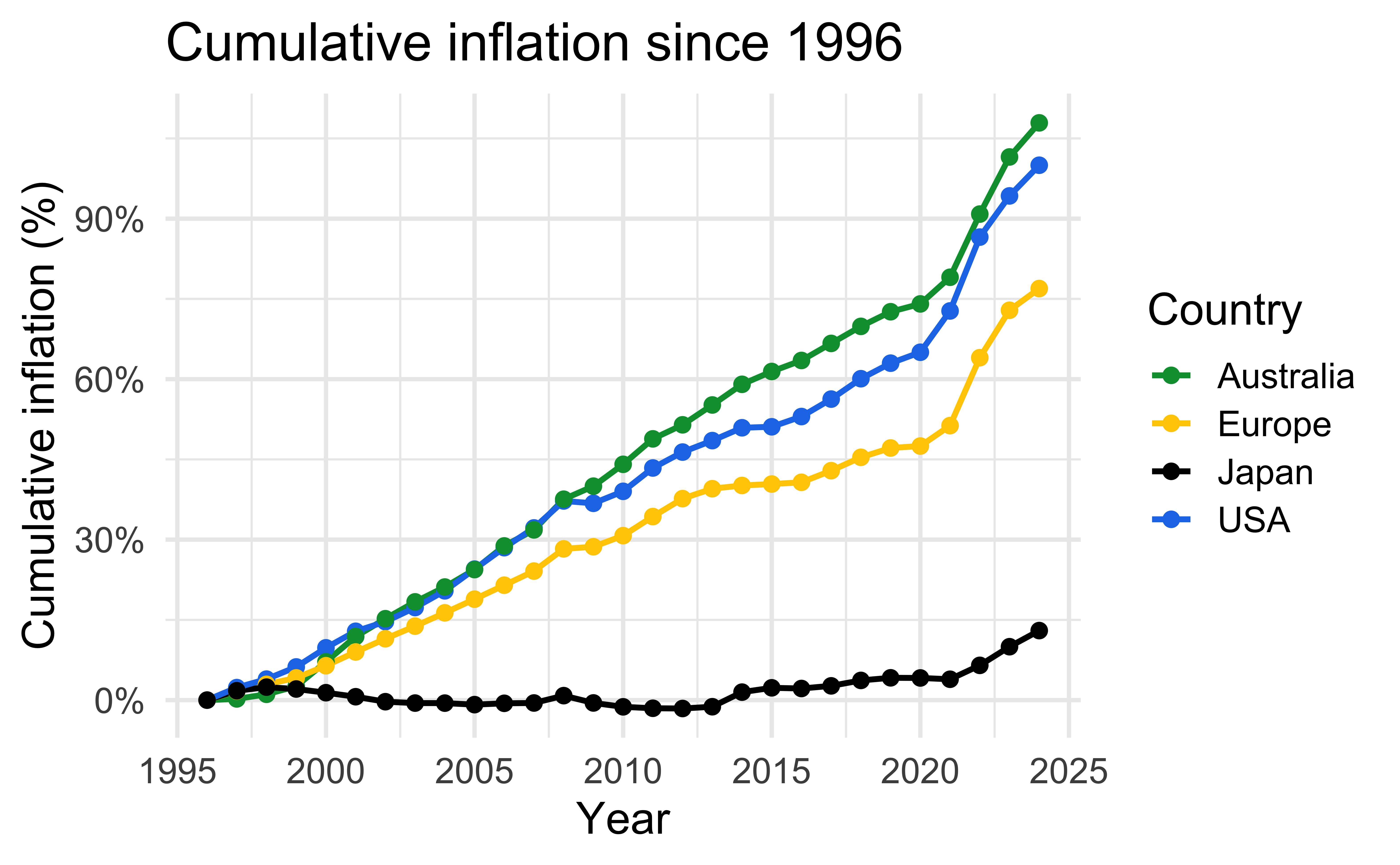
Static plot (excluding Turkiye)
inflation_long |>
  filter(country != "Turkiye") |>
  ggplot(aes(x = year, y = cumulative_pct, color = country)) +
  geom_line(linewidth = 1) +
  geom_point(size = 2) +
  scale_color_manual(values = flag_colors) +
  scale_y_continuous(labels = label_comma(suffix = "%")) +
  labs(
    title = "Cumulative inflation since 1996",
    x = "Year",
    y = "Cumulative inflation (%)",
    color = "Country"
  )
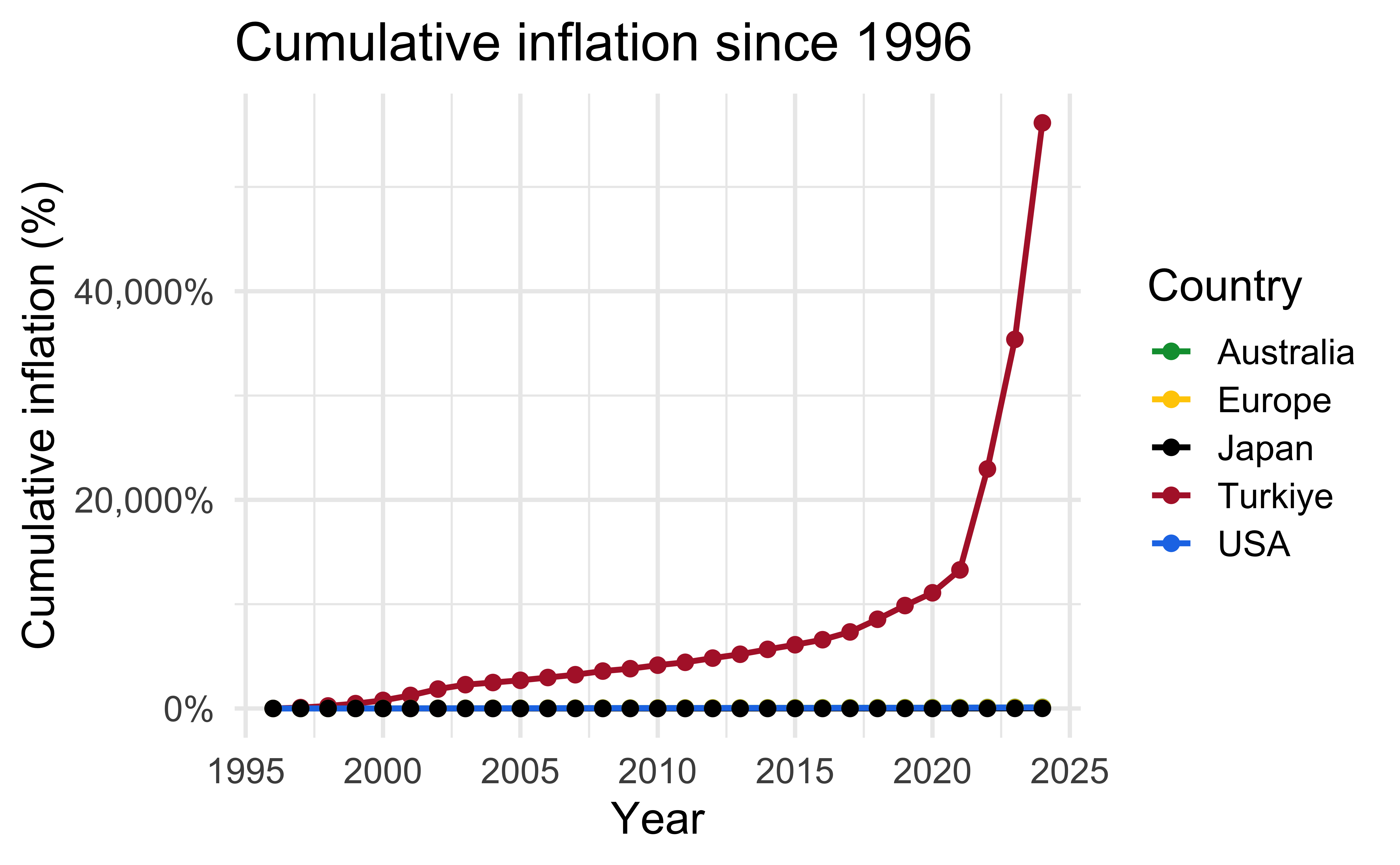
Static plot (with Turkiye)
inflation_long |>
  ggplot(aes(x = year, y = cumulative_pct, color = country)) +
  geom_line(linewidth = 1) +
  geom_point(size = 2) +
  scale_color_manual(values = flag_colors) +
  scale_y_continuous(labels = label_comma(suffix = "%")) +
  labs(
    title = "Cumulative inflation since 1996",
    x = "Year",
    y = "Cumulative inflation (%)",
    color = "Country"
  )
Animate
inflation_long |>
  ggplot(
    aes(
      x = year,
      y = cumulative_pct,
      color = country,
      group = country
    )
  ) +
  geom_line(linewidth = 1) +
  geom_point(size = 2) +
  scale_color_manual(values = flag_colors) +
  scale_y_continuous(labels = label_comma(suffix = "%")) +
  labs(
    title = "Cumulative inflation since 1996",
    subtitle = "Year: {round(frame_along)}",
    x = "Year",
    y = "Cumulative inflation (%)",
    color = "Country"
  ) +
  transition_reveal(year)
Animate with expanding y-axis
inflation_long |>
  ggplot(
    aes(
      x = year,
      y = cumulative_pct,
      color = country,
      group = country
    )
  ) +
  geom_line(linewidth = 1) +
  geom_point(size = 2) +
  scale_color_manual(values = flag_colors) +
  scale_y_continuous(labels = label_comma(suffix = "%")) +
  labs(
    title = "Cumulative inflation since 1996",
    subtitle = "Year: {round(frame_along)}",
    x = "Year",
    y = "Cumulative inflation (%)",
    color = "Country"
  ) +
  transition_reveal(year) +
  view_follow(fixed_x = TRUE)
Transitions
Which transition was used in the following animations?
![]()
transition_layers()
New layers are being added (and removed) over the dots.
Views
Which view was used in the following animations?
view_follow()
Plot axis follows the range of the data.
Shadows
Which shadow was used in the following animations?
shadow_wake()
The older tails of the points shrink in size, leaving a “wake” behind it.
Shadows
Which shadow was used in the following animations?
shadow_mark()
Permanent marks are left by previous points in the animation.
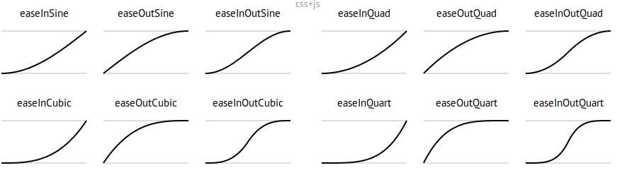
Animation controls
How data moves from one position to another.
A not-so-simple example
Pass in the dataset to ggplot

A not-so-simple example
For each dataset we have x and y values, in addition we can map dataset to color
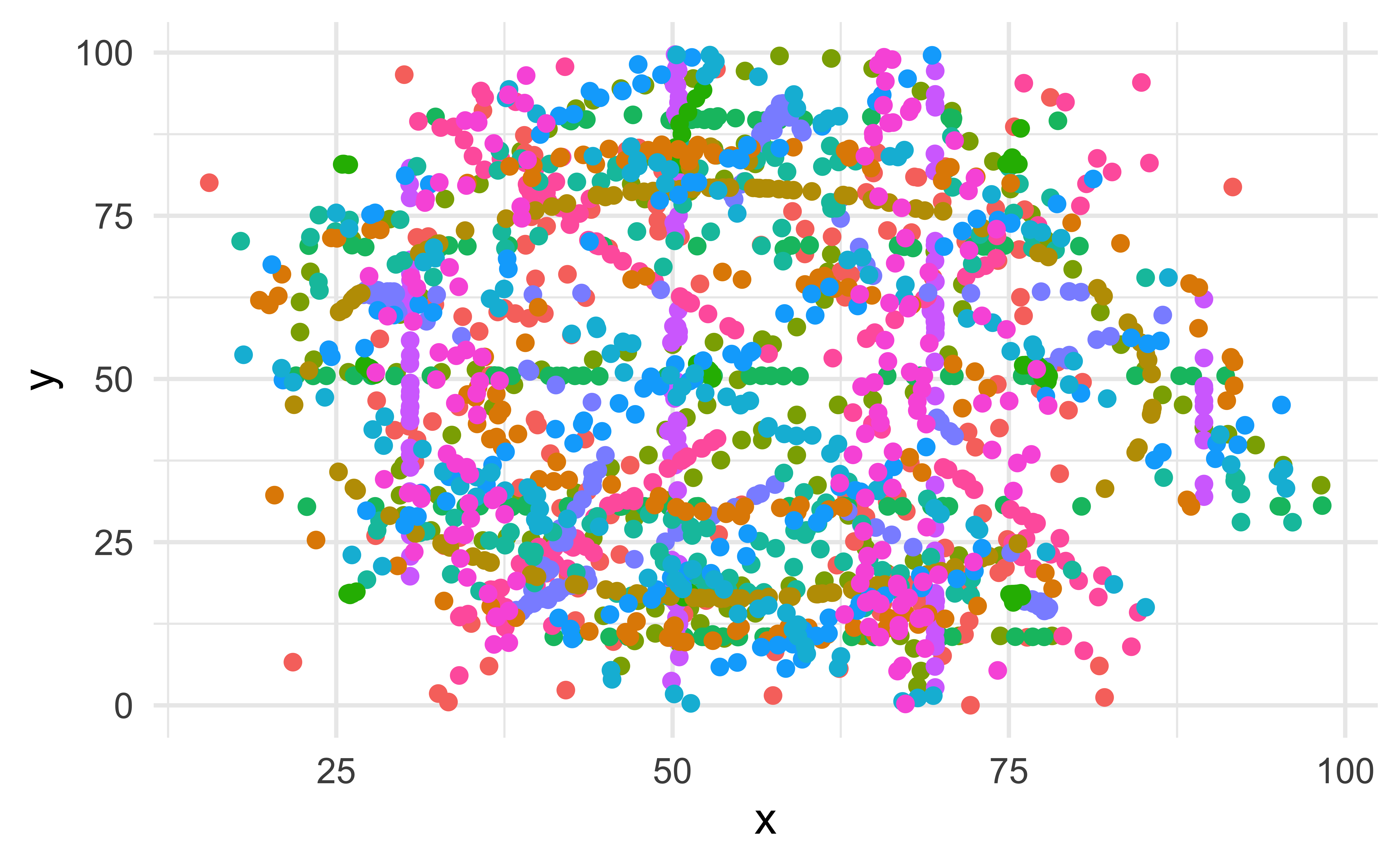
A not-so-simple example
Trying a simple scatter plot first, but there is too much information
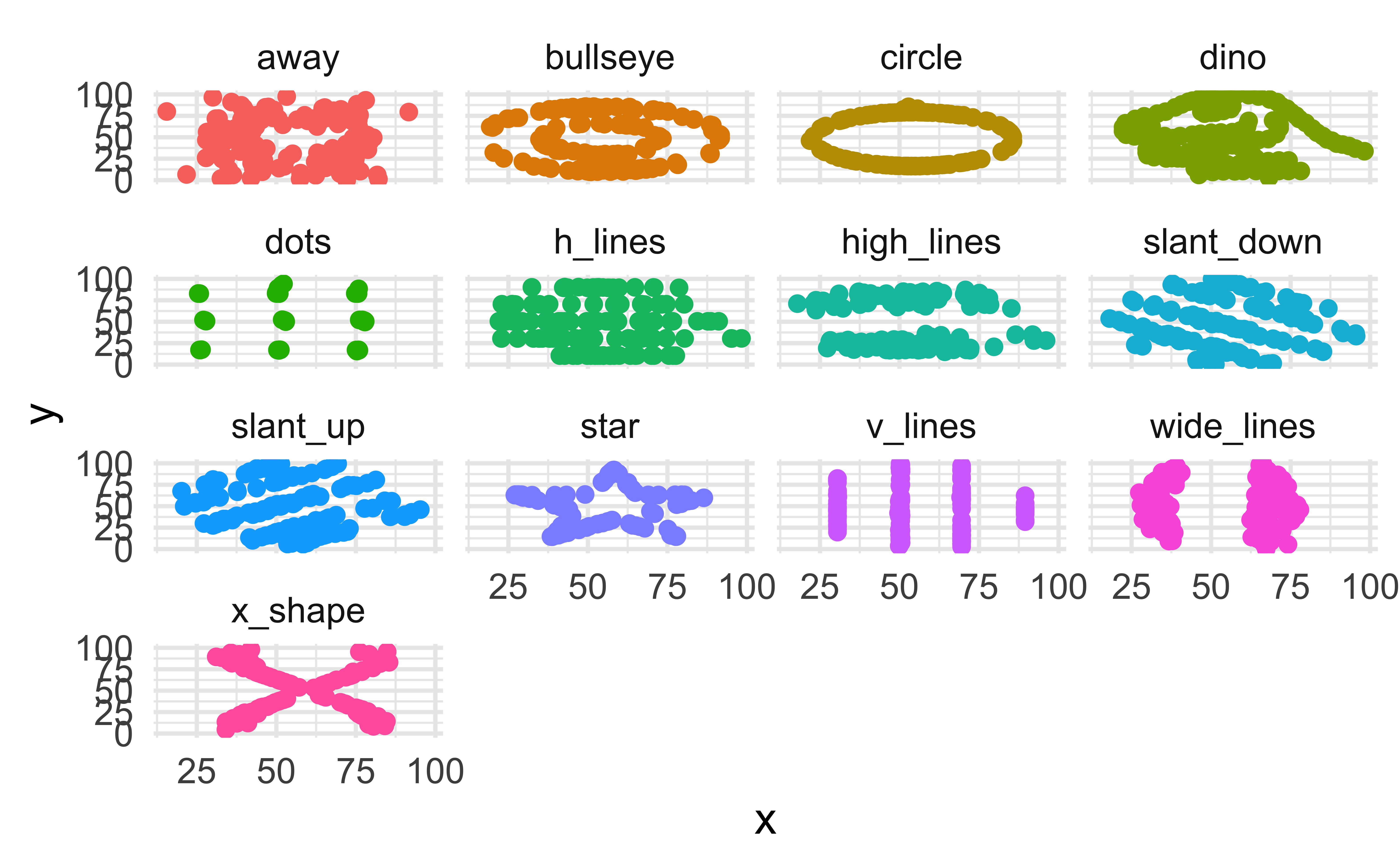
A not-so-simple example
We can use facets to split up by dataset, revealing the different distributions
A not-so-simple example