# load packages
library(tidyverse)

# set theme for ggplot2
ggplot2::theme_set(ggplot2::theme_minimal(base_size = 16))

# set figure parameters for knitr
knitr::opts_chunk$set(
  fig.width = 7, # 7" width
  fig.asp = 0.618, # the golden ratio
  fig.retina = 3, # dpi multiplier for displaying HTML output on retina
  fig.align = "center", # center align figures
  dpi = 300 # higher dpi, sharper image
)Graphical perception
Lecture 24
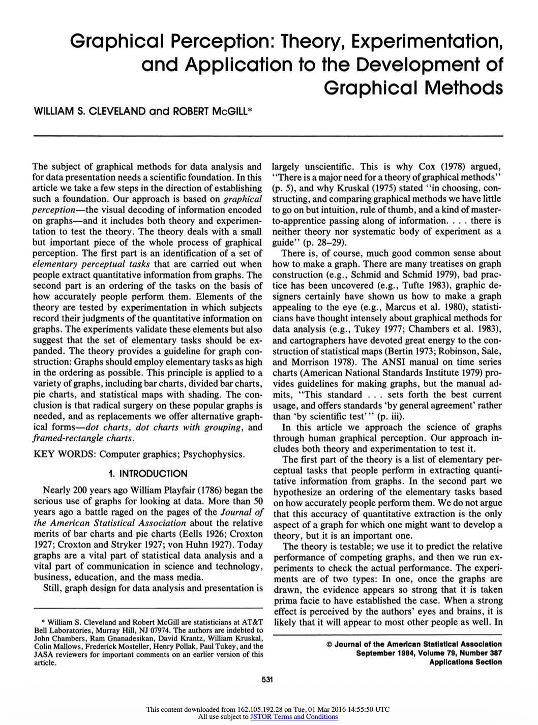
Cleveland & McGill (1984)
“Graphical Perception: Theory, Experimentation, and Application to the Development of Graphical Methods”
Journal of the American Statistical Association
- William S. Cleveland and Robert McGill (AT&T Bell Labs)
- One of the most influential papers in data visualization
- Established empirical foundations for graph design
- Over 2,800 citations
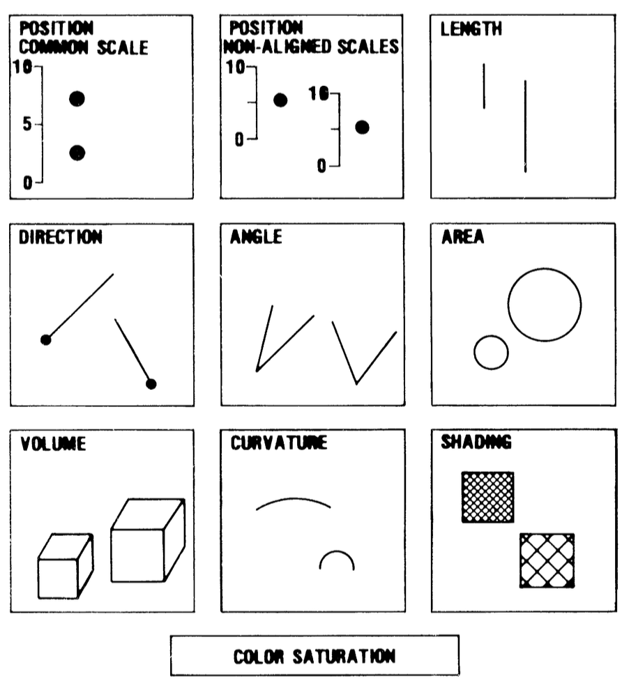
10 Elementary perceptual tasks
Cleveland & McGill identified 10 basic visual tasks people use to extract quantitative information from graphs:
Get ready to answer some questions!
https://app.wooclap.com/STA313S26

Question 1
Which of the following is true?
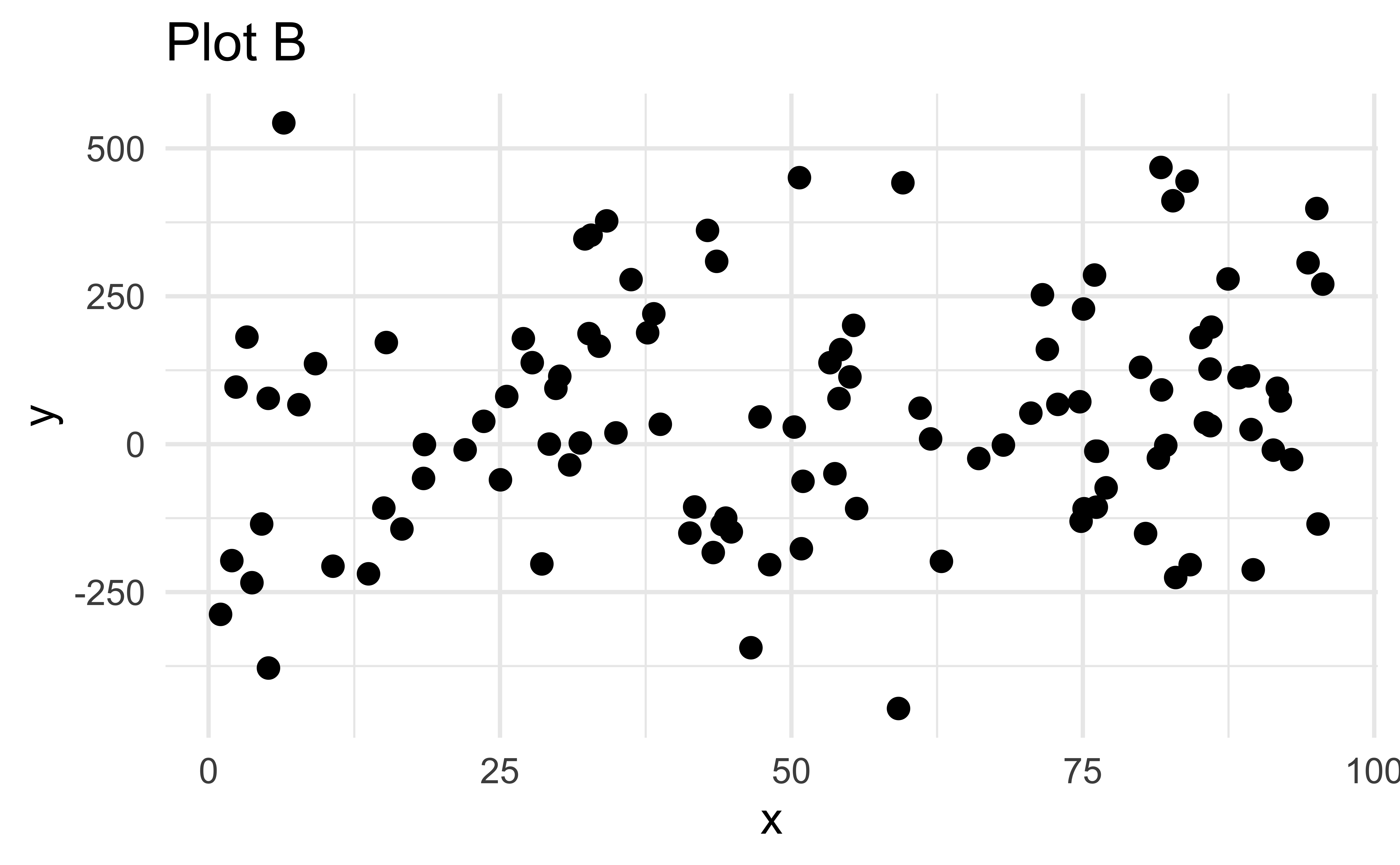
- Plot A has more points than Plot B
- Plot B has more points than Plot A
- Plot A and Plot B have the same number of points

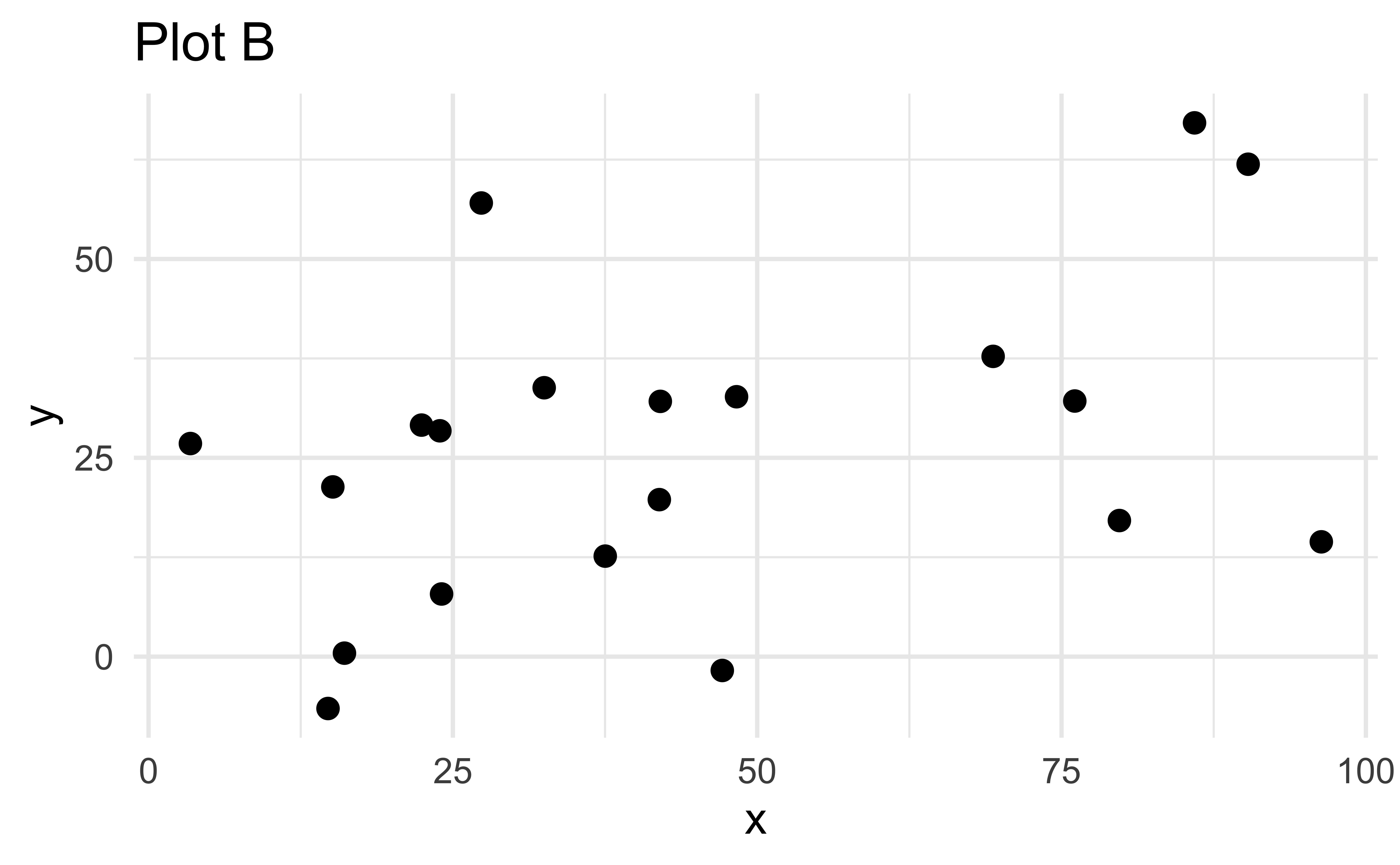
Question 2
Which of the following is true?
- Plot A has more points than Plot B
- Plot B has more points than Plot A
- Plot A and Plot B have the same number of points

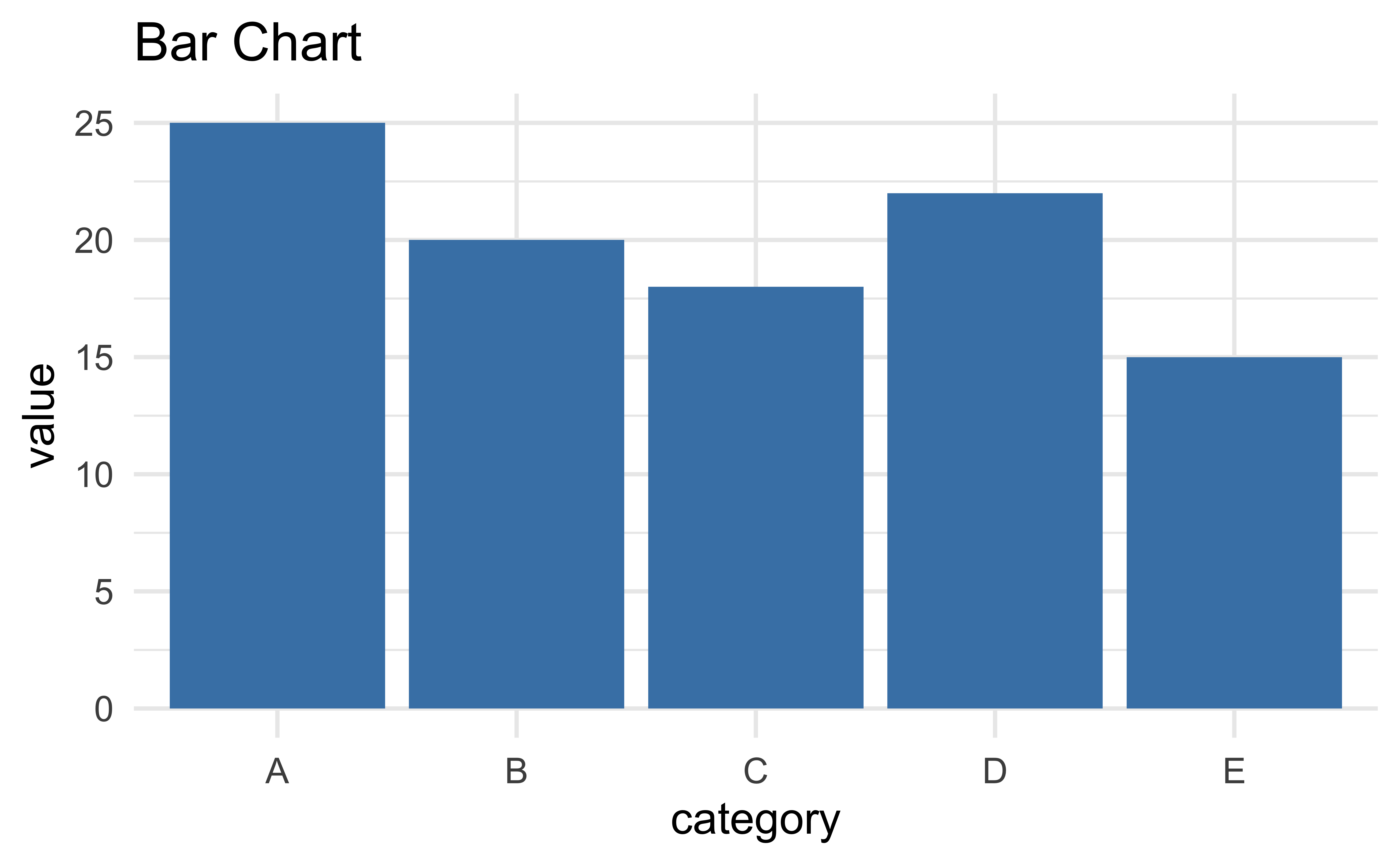
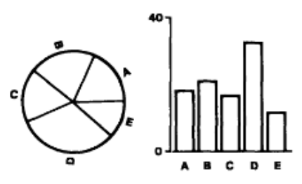
Example: Bar chart vs. Pie chart
Bar chart
- Primary task: Position along common scale
- High accuracy
- Easy to compare values
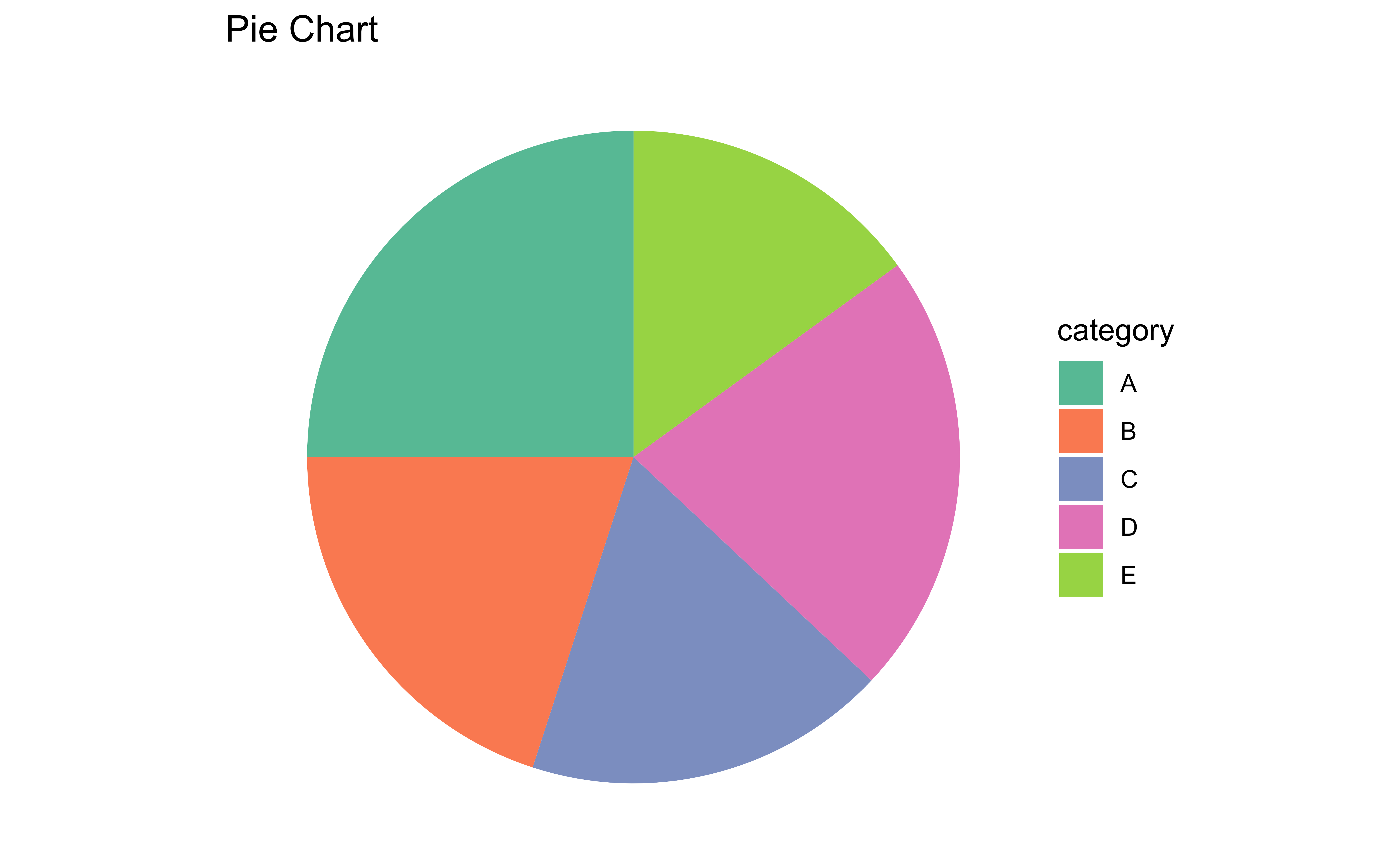
Pie chart
- Primary task: Angle judgment
- Lower accuracy
- Harder to compare non-adjacent slices
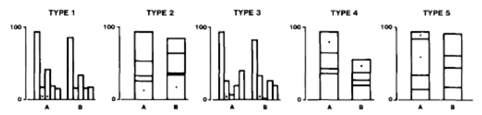
Experiment 1: Position-length
- 55 subjects judged divided bar charts
- 5 types of bar chart configurations
- Tasks:
- Which of the two indicated (with a dot) bars or two segments is smaller?
- What percentage is the smaller of the larger?
Experiment 2: Position-angle
- 54 subjects judged pie charts vs. bar charts
- 10 sets of values, each shown as pie and bar
- Tasks:
- Which bar or segment is largest?
- What percentage each of the other four values is of the largest bar or segment?
Experiment results
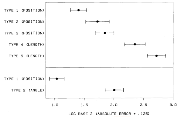
Position-length: Average errors for length judgments are considerably larger than those for position judgments.
Position-angle: Average errors for angle judgments is considerably larger than for position judgments.
Practice: Bar chart

Which is smaller? What % is it of the larger?
Trial 1: Bar chart
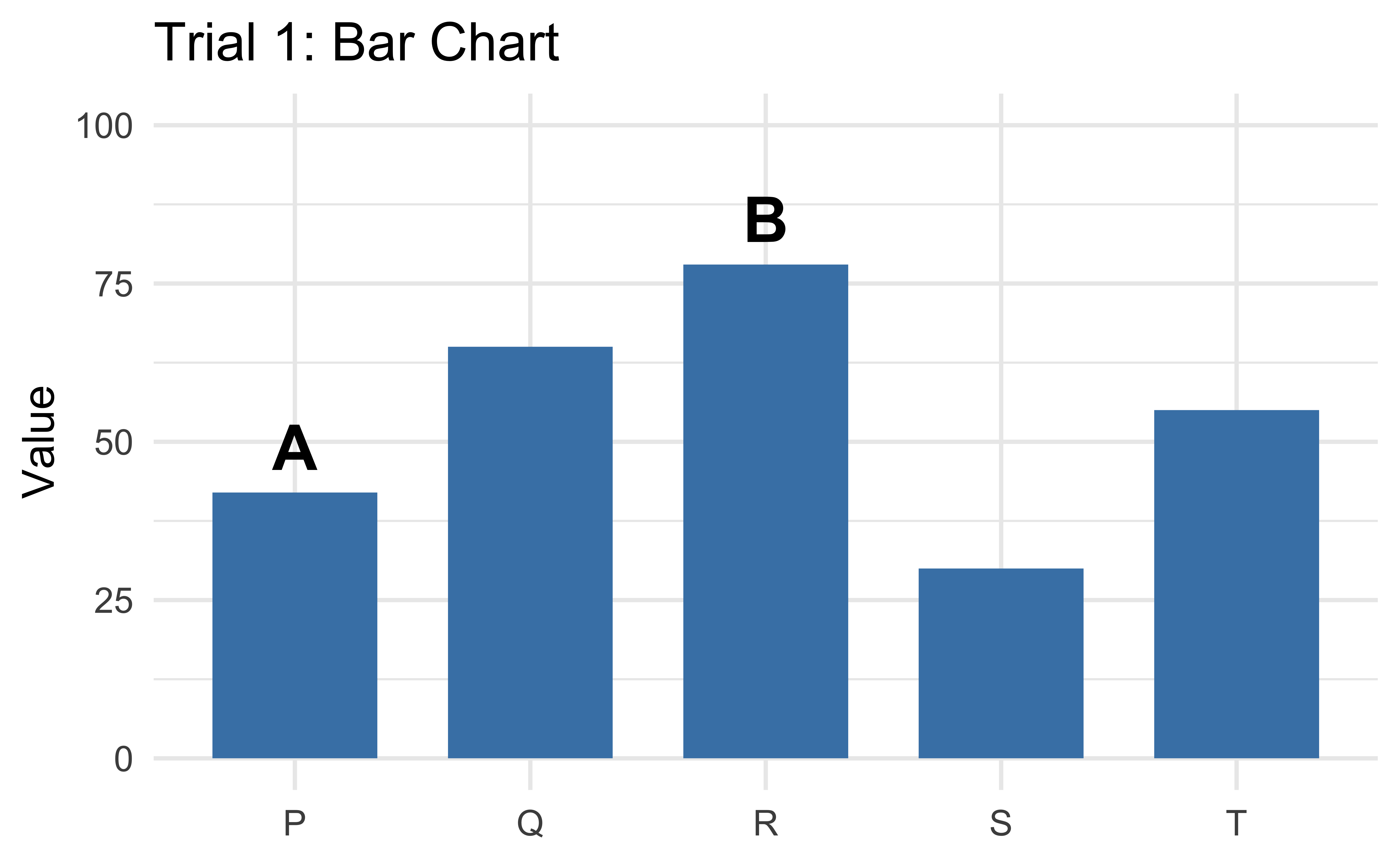
Record: Smaller = ___ | Estimate = ____%
Trial 2: Bar chart

Record: Smaller = ___ | Estimate = ____%
Trial 3: Pie chart

Record: Smaller = ___ | Estimate = ____%
Trial 4: Pie chart

Record: Smaller = ___ | Estimate = ____%
Trial 5: Bubble chart

Record: Smaller = ___ | Estimate = ____%
Trial 6: Bubble chart

Record: Smaller = ___ | Estimate = ____%
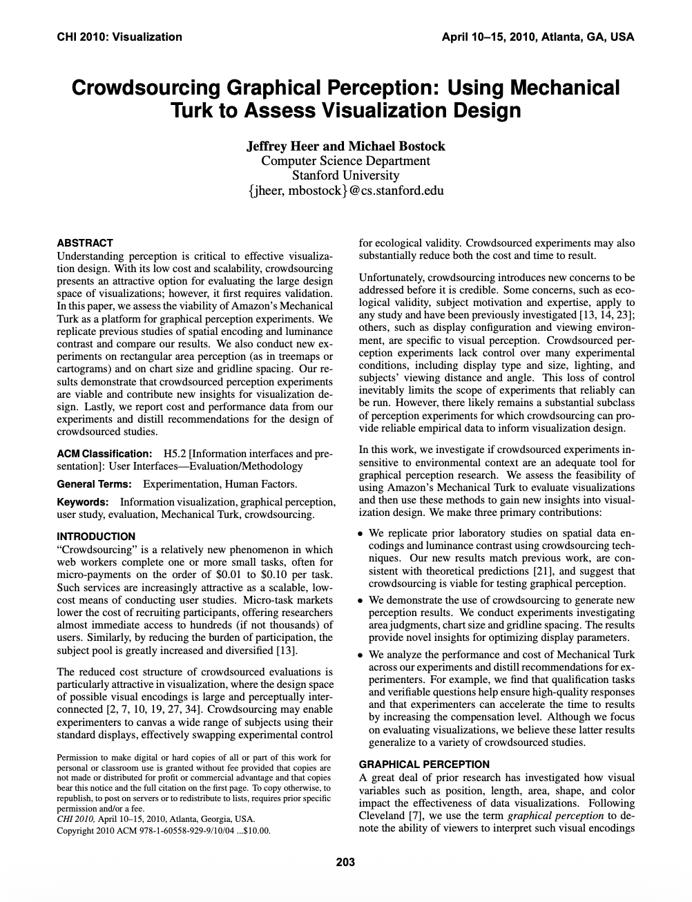
Crowdsourcing graphical perception
26 years later…
Jeffrey Heer and Michael Bostock (Stanford) replicated Cleveland & McGill using Amazon Mechanical Turk.
Why replicate?
- Test if crowdsourcing is viable for perception experiments
- Extend to new chart types (treemaps, bubble charts)
- Larger, more diverse subject pool
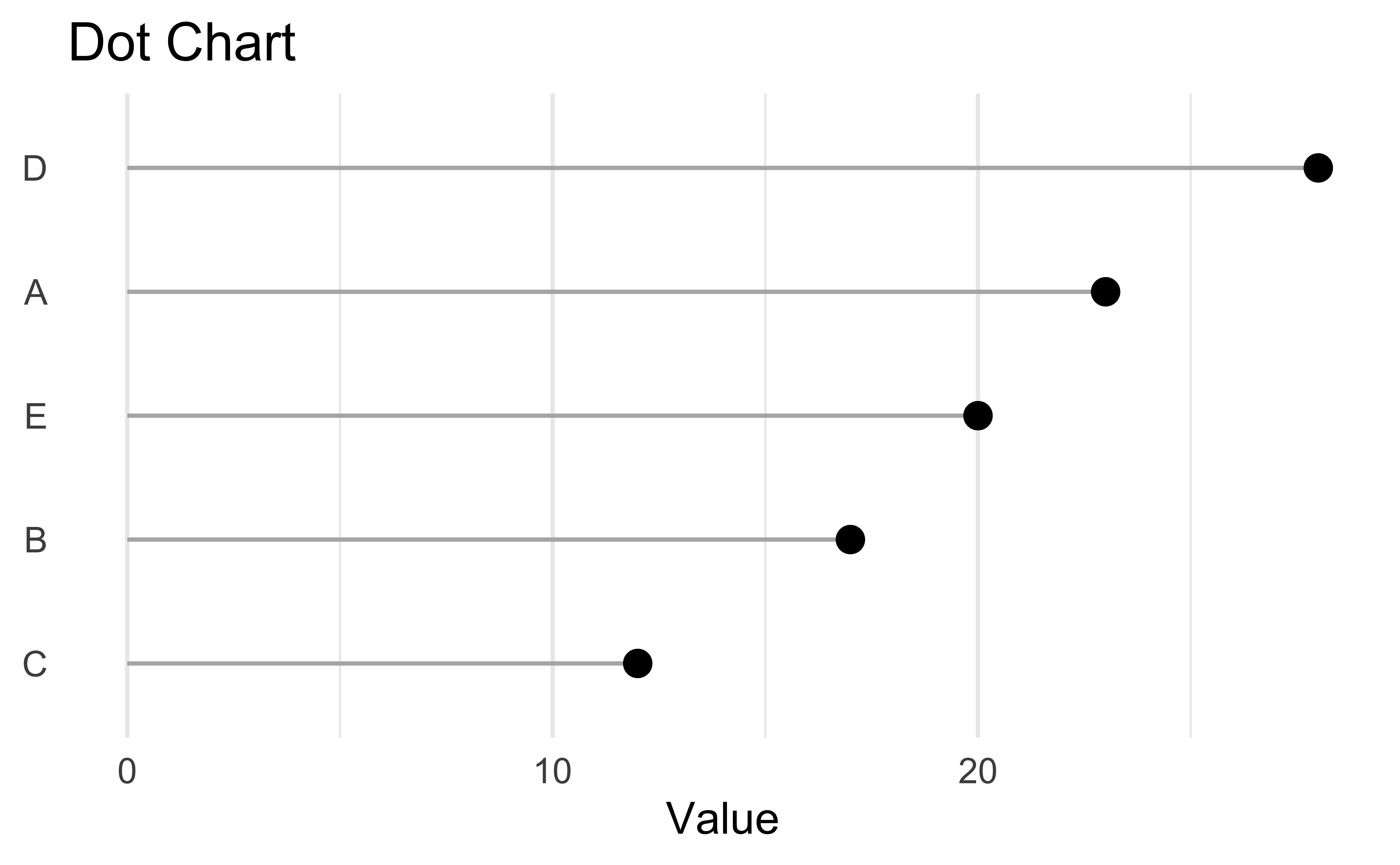
Dot (lollipop) chart: A Cleveland favorite