Data visualization with Python I

Lecture 22

Dr. Mine Çetinkaya-Rundel

Duke University
STA 313 - Spring 2026

Warm up

Announcements

Mini-project 2 due today at 5 pm
Project 2 peer evaluation 1 due Wednesday at 5 pm – no extensions as we’d like to share summaries before lab the next day
Project 2 presentation schedule: https://vizdata.org/projects/project-2.html#due-dates
Upcoming HW deadlines:
- HW 5 due Monday, April 20 at 5 pm
- HW 6 (optional) due Tuesday, April 28 at 5 pm

SSMU event: “Existential crisis! Is my degree worthless?” with Mr. Davis Vaughan

Join SSMU for a seminar featuring Davis Vaughan, a software engineer at Posit, as he asks the timely question: is YOUR degree worth it?! Davis works on Positron, a data science-focused IDE, as well as the R packages that make up the tidyverse. He will walk through examples of how he and his colleagues use Claude Code and other AI tools to amplify their own skills, rather than replace them.

🗓️ 4:30 PM-5:30 PM on Wednesday, April 8th
📍 Old Chem 116

From last time: Generative art resources

R packages:
- aRtsy by Koen Derks
- generativeart by Katharina Brunner
- flametree and jasmines bu Danielle Navarro
- ambient and particles by Thomas Lin Pedersen
More aRtists: rtistry art gallery by Ijeamaka Anyene
A whole course on Generative Art by Danielle Navarro: https://art-from-code.netlify.app

Setup

library(tidyverse)

Python:

import polars as pl
from plotnine import ggplot, aes, geom_point, geom_segment, labs, theme, theme_minimal

Data visualization with Python

Spot the difference

Plot A:

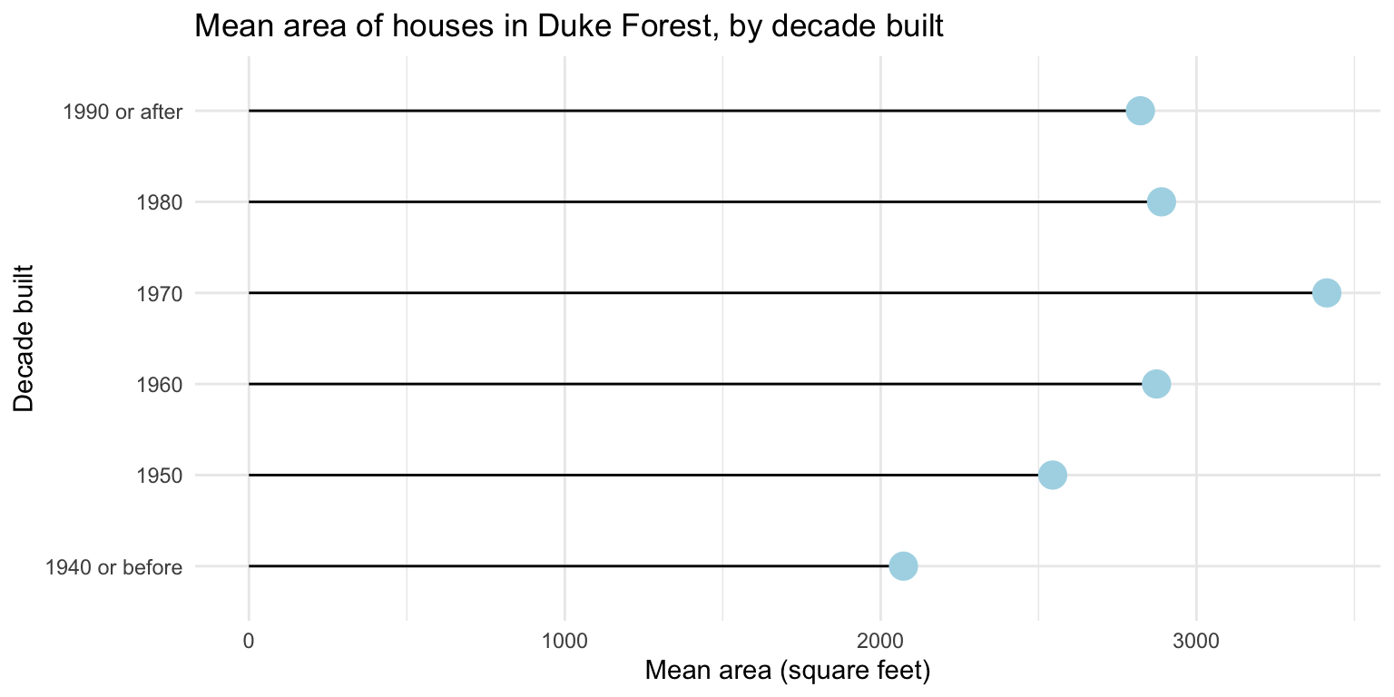
Plot B:

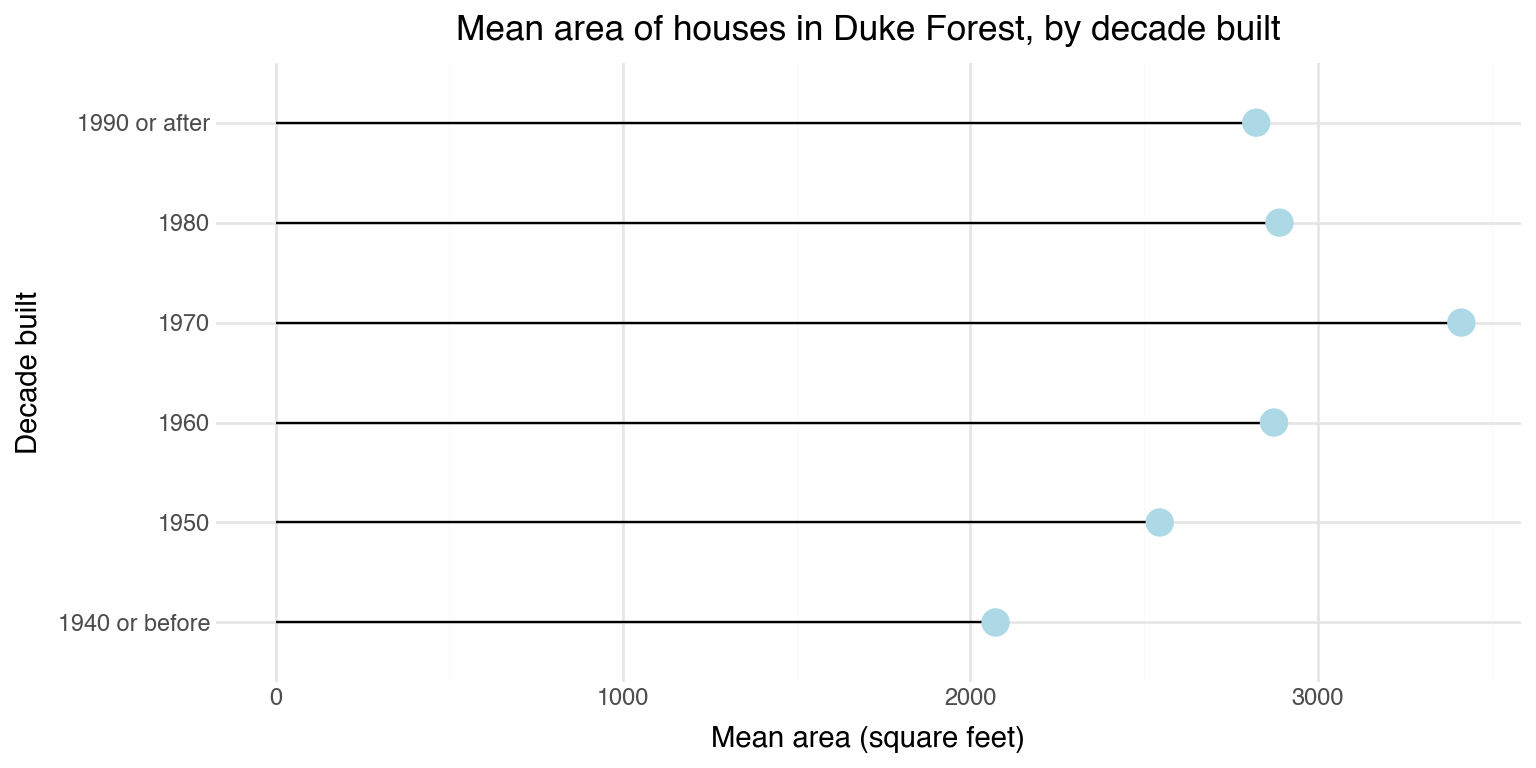
Spot the difference

Plot A:

Plot B:

Overview

Goal:
- Get a taste of data visualization with Python with plotnine – a Python data visualization package based on the grammar of graphics and inspired by ggplot2 – and do so in Positron using uv for package management.
- Not: A comprehensive introduction to Python or even to data visualization with Python.
- Not: Tips and tricks for working with Python outside of Positron.
Approach:
- We will cover the basics of plotnine and how to create different types of plots.
- We will use polars to read in data from CSV files, but we will not cover how to prepare your data for visualization in Python.

But…

there are some Python details we can’t avoid…

Package management
in Python with `uv`

Python packaging landscape

Python’s packaging ecosystem has historically been fragmented:

Multiple tools: pip, virtualenv, venv, conda, poetry, pipenv, etc.
Multiple config files: requirements.txt, setup.py, pyproject.toml, etc.
Version management often handled separately (pyenv)

uv is a modern tool that aims to unify these concerns with a fast, Rust-based implementation.

What is uv?

uv is a Python package and project manager developed by Astral.

Key features:

Extremely fast (10-100x faster than pip)
Manages Python versions
Creates and manages virtual environments
Installs packages
Handles project dependencies via pyproject.toml
Drop-in replacement for pip and virtualenv
Directly supported by Positron and Reticulate

Installing uv

uv is already installed on the departmental servers, for local installs:

On MacOS/Linux:

curl -LsSf https://astral.sh/uv/install.sh | sh

or with homebrew:

brew install uv

or with pip / pipx

pipx install uv
pip install uv

Verify installation

Once installed you should be able to run the following,

uv --version

uv 0.11.3 (Homebrew 2026-04-01 aarch64-apple-darwin)

As long as you have something higher than 0.9.* you should be fine.

Managing Python versions

uv can install and manage multiple Python versions,

uv python install 3.14

Python 3.14 is already installed

uv python pin 3.14

Pinned `.python-version` to `3.14`

The pinned version is stored in ~/.python-version and will be used automatically.

Initializing a project

Use uv init to create a new project,

mkdir my-project
cd my-project
uv init

Initialized project `my-project`

ls -la

total 32
drwxr-xr-x   8 mine  staff   256 Apr  6 00:22 .
drwx------@ 55 mine  staff  1760 Apr  6 00:22 ..
drwxr-xr-x@  9 mine  staff   288 Apr  6 00:22 .git
-rw-r--r--@  1 mine  staff   109 Apr  6 00:22 .gitignore
-rw-r--r--@  1 mine  staff     5 Apr  6 00:22 .python-version
-rw-r--r--@  1 mine  staff    88 Apr  6 00:22 main.py
-rw-r--r--@  1 mine  staff   156 Apr  6 00:22 pyproject.toml
-rw-r--r--@  1 mine  staff     0 Apr  6 00:22 README.md

This creates a pyproject.toml, a sample main.py script, and basic git infrastructure. Generally, we only really care about the pyproject.toml which we can exclusively generate via uv init --bare.

`pyproject.toml`

Modern project metadata file, tracks python version and package dependencies among other details.

[project]
name = "my-project"
version = "0.1.0"
description = "Add your description here"
readme = "README.md"
requires-python = ">=3.14"
dependencies = []

Adding dependencies

Once we have our project setup we can add (and install) dependencies directly via uv. uv add updates pyproject.toml and installs the package (creating a venv if needed).

uv add plotnine

Using CPython 3.14.3
Creating virtual environment at: .venv
Resolved 19 packages in 188ms
Installed 17 packages in 134ms
 + contourpy==1.3.3
 + cycler==0.12.1
 + fonttools==4.62.1
 + kiwisolver==1.5.0
 + matplotlib==3.10.8
 + mizani==0.14.4
 + numpy==2.4.4
 + packaging==26.0
 + pandas==3.0.2
 + patsy==1.0.2
 + pillow==12.2.0
 + plotnine==0.15.3
 + pyparsing==3.3.2
 + python-dateutil==2.9.0.post0
 + scipy==1.17.1
 + six==1.17.0
 + statsmodels==0.14.6

uv add polars

Resolved 21 packages in 142ms
Installed 2 packages in 6ms
 + polars==1.39.3
 + polars-runtime-32==1.39.3

Updated `pyproject.toml`

[project]
name = "my-project"
version = "0.1.0"
description = "Add your description here"
readme = "README.md"
requires-python = ">=3.14"
dependencies = [
    "plotnine>=0.15.3",
    "polars>=1.39.3",
]

Virtual environments

Virtual environments isolate project dependencies from the system Python and other projects. Packages are installed in a local folder in your project.

As we just saw, using uv add will create a new virtual environment in .venv by default if there is not an existing venv.

Activating environments in Positron with uv

Positron automatically detects virtual environments in your project directory. When you open a folder containing a .venv directory (created by uv), Positron will:

Detect the environment and offer to use it
Show the active Python interpreter in the status bar
Use the environment for the Python console and when running scripts

If not automatically detected, you can manually select the interpreter via the Command Palette (Cmd+Shift+P / Ctrl+Shift+P) and searching for “Python: Select Interpreter”.

`uv sync`

Since the .venv folder is system specific (and large) it is not typically committed to git. Instead you will likely clone a repository that just has a pyproject.toml file.

Use uv sync to construct the venv and install all dependencies for the project.

Common workflows

New project setup:

mkdir my-project # or use Positron's new project wizard
cd my-project    # and navigate to the project folder
uv init --bare
uv add plotine polars

Clone existing project:

git clone <repo-url> # or use Positron's git integration
cd <repo>            # and navigate to the project folder
uv sync

Let’s give it a try!

Go to ae-16 and let’s make a simple plot with plotnine!

For now, ae-16-Python.qmd only.

Introduction to plotnine

What is plotnine?

plotnine is a Python visualization library that implements the grammar of graphics.

Based on the same principles as ggplot2 in R
Enables data visualization through composable, layered components
Maps data to visual properties systematically
Works with Pandas and Polars DataFrames

The grammar of graphics

A plot is built from layers of components:

Component	Description
Data	The dataset to visualize
Aesthetics	Mappings from data to visual properties
Geoms	Geometric objects that represent data
Scales	Control how data values map to visual values
Facets	Split data into multiple subplots
Coords	Coordinate system for the plot
Themes	Control non-data visual elements

Data

All plots begin with passing data to ggplot():

from plotnine import ggplot

(
    ggplot(data=my_dataframe)
)

Tip

Plotnine works best with tidy data:

Each variable is a column
Each observation is a row
Each type of observational unit is a table

Aesthetic mappings

The aes() function maps data columns to visual properties:

from plotnine import ggplot, aes

ggplot(df, aes(x="column1", y="column2"))

Common aesthetic mappings:

Aesthetic	Description
`x`, `y`	Position on axes
`color`	Color of points/lines
`fill`	Fill color of shapes
`size`	Size of points
`shape`	Shape of points
`alpha`	Transparency

Geometric objects (geoms)

from plotnine import ggplot, aes, geom_point

(
    ggplot(df, aes(x="x_var", y="y_var")) 
    + geom_point()
)

Note

In Python, wrap the entire plot expression in parentheses () to allow line breaks.

Geometric objects (geoms)

Geoms determine how data is visually represented:

Geom	Description
`geom_point()`	Scatter plot
`geom_line()`	Line plot
`geom_bar()`	Bar chart
`geom_histogram()`	Histogram
`geom_boxplot()`	Box plot
`geom_smooth()`	Smoothed line
`geom_text()`	Text labels
`geom_segment()`	Line segments
`geom_area()`	Area plot
`geom_density()`	Density plot

Layering with `+`

Components are combined using the + operator:

from plotnine import ggplot, aes, geom_point, geom_smooth

(
    ggplot(df, aes(x="x_var", y="y_var"))
    + geom_point()
    + geom_smooth(method="lm")
)

Note

In Python, move the + to the start of the line and add a line break before +.

Scales

Scales customize how data values map to visual values.

Naming pattern: scale_<aesthetic>_<type>

from plotnine import ggplot, aes, geom_point, scale_color_continuous

(
    ggplot(df, aes(x="x_var", y="y_var", color="z_var"))
    + geom_point()
    + scale_color_continuous(cmap_name="viridis")
)

Common scale functions:

scale_x_continuous(), scale_y_continuous() - continuous axes
scale_x_log10(), scale_y_log10() - log-transformed axes
scale_color_manual(), scale_fill_manual() - custom colors
scale_color_brewer(), scale_fill_brewer() - ColorBrewer palettes

Facets

Facets split data into multiple subplots:

facet_wrap() - wraps panels into rows

from plotnine import facet_wrap

(
    ggplot(df, aes(x="x", y="y"))
    + geom_point()
    + facet_wrap("~category")
)

facet_grid() - creates a grid of panels

from plotnine import facet_grid

(
    ggplot(df, aes(x="x", y="y"))
    + geom_point()
    + facet_grid("row_var ~ col_var")
)

Coordinate systems

Coordinate functions specify the plot’s coordinate system:

from plotnine import coord_fixed, coord_cartesian, coord_trans

# Equal aspect ratio
ggplot(...) + coord_fixed()

# Zoom without clipping data
ggplot(...) + coord_cartesian(xlim=(0, 10))

# Transformed cartesian coordinate system
ggplot(...) + coord_trans()

Themes

Themes control non-data visual elements like fonts, colors, and grid lines.

Pre-built themes:

from plotnine import theme_minimal, theme_bw, theme_classic

ggplot(...) + theme_minimal()
ggplot(...) + theme_bw()
ggplot(...) + theme_classic()

Custom theme adjustments:

from plotnine import theme, element_text, element_line

(
    ggplot(...)
    + theme_minimal()
    + theme(
        axis_text=element_text(size=12),
        legend_position="bottom",
        figure_size=(10, 6)
    )
)

Labels

Use labs() to add titles and axis labels:

from plotnine import labs

(
    ggplot(df, aes(x="x_var", y="y_var"))
    + geom_point()
    + labs(
        title="My Plot Title",
        subtitle="A descriptive subtitle",
        x="X Axis Label",
        y="Y Axis Label",
        color="Legend Title"
    )
)

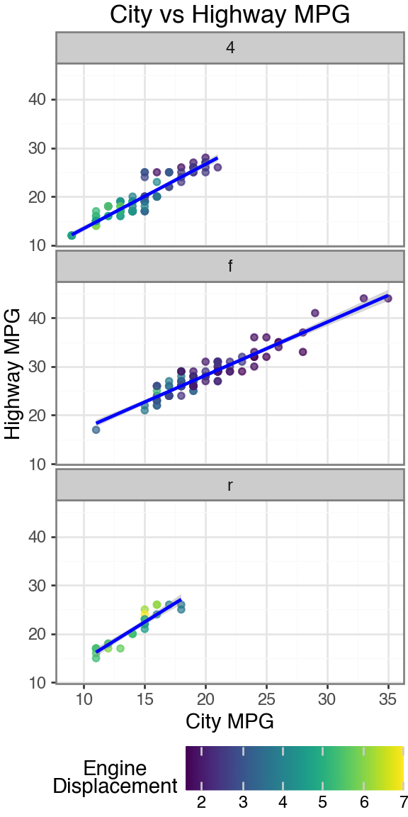
Putting it all together

from plotnine import *
from plotnine.data import mpg

(
    ggplot(mpg, aes(x="cty", y="hwy"))
    + geom_point(aes(color="displ"), alpha=0.7)
    + geom_smooth(method="lm", color="blue")
    + scale_color_continuous(cmap_name="viridis")
    + facet_wrap("~drv", ncol=1)
    + labs(
        title="City vs Highway MPG",
        x="City MPG",
        y="Highway MPG",
        color="Engine\nDisplacement"
    )
    + theme_bw()
    + theme(
        figure_size=(3, 6), 
        legend_position="bottom"
    )
)

Key differences from ggplot2

ggplot2 (R)	plotnine (Python)
`aes(x = var)`	`aes(x="var")` (quoted strings)
`+` at end of line	`+` at start of line (inside parens)
`theme(legend.position = ...)`	`theme(legend_position=...)` (underscores)
No parens needed	Wrap in `()` for multi-line plots
`ggsave()`	`.save()` method on plot object

# Saving a plot
p = ggplot(...) + geom_point()
p.save("my_plot.png", width=10, height=6, dpi=300)

Back to `ae-16`

Go to ae-16 and work on ae-16-R-and-Python.qmd.

Data visualization with Python I

Warm up

Announcements

SSMU event: “Existential crisis! Is my degree worthless?” with Mr. Davis Vaughan

From last time: Generative art resources

Setup

Data visualization with Python

Spot the difference

Spot the difference

Overview

But…

Package management in Python with uv

Python packaging landscape

What is uv?

Installing uv

Verify installation

Managing Python versions

Initializing a project

pyproject.toml

Adding dependencies

Updated pyproject.toml

Virtual environments

Activating environments in Positron with uv

uv sync

Common workflows

Let’s give it a try!

Introduction to plotnine

What is plotnine?

The grammar of graphics

Data

Aesthetic mappings

Geometric objects (geoms)

Geometric objects (geoms)

Layering with +

Scales

Facets

Coordinate systems

Themes

Labels

Putting it all together

Key differences from ggplot2

Back to ae-16

Package management
in Python with `uv`

`pyproject.toml`

Updated `pyproject.toml`

`uv sync`

Layering with `+`

Back to `ae-16`