# load packages
library(openintro)
library(tidyverse)
library(tidymodels)
library(ggdist)

# set theme for ggplot2
ggplot2::theme_set(ggplot2::theme_bw(base_size = 16))

# set figure parameters for knitr
knitr::opts_chunk$set(
  fig.width = 7, # 7" width
  fig.asp = 0.618, # the golden ratio
  fig.retina = 3, # dpi multiplier for displaying HTML output on retina
  fig.align = "center", # center align figures
  dpi = 300 # higher dpi, sharper image
)
Visualizing uncertainty II
Lecture 17
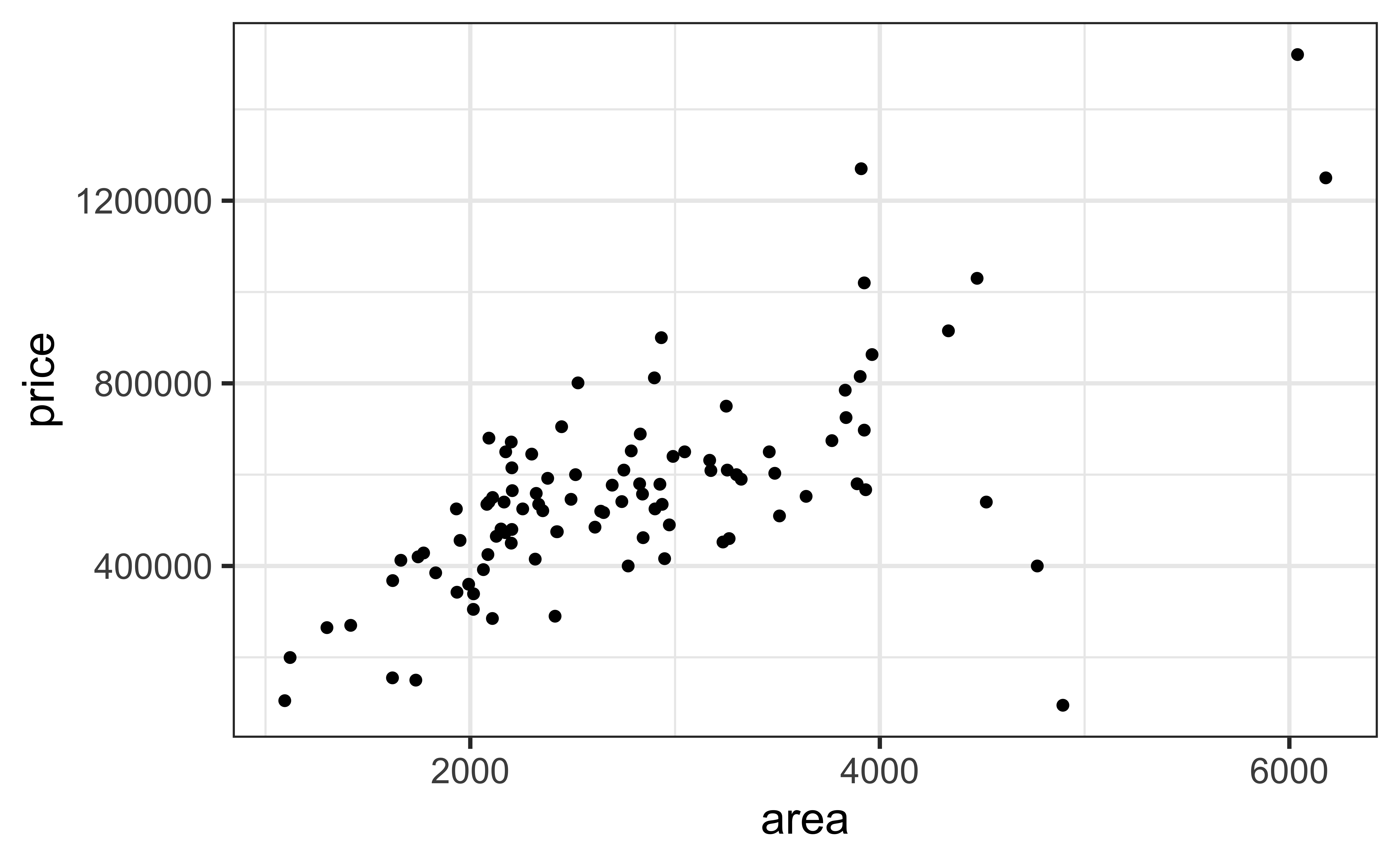
Price vs. area
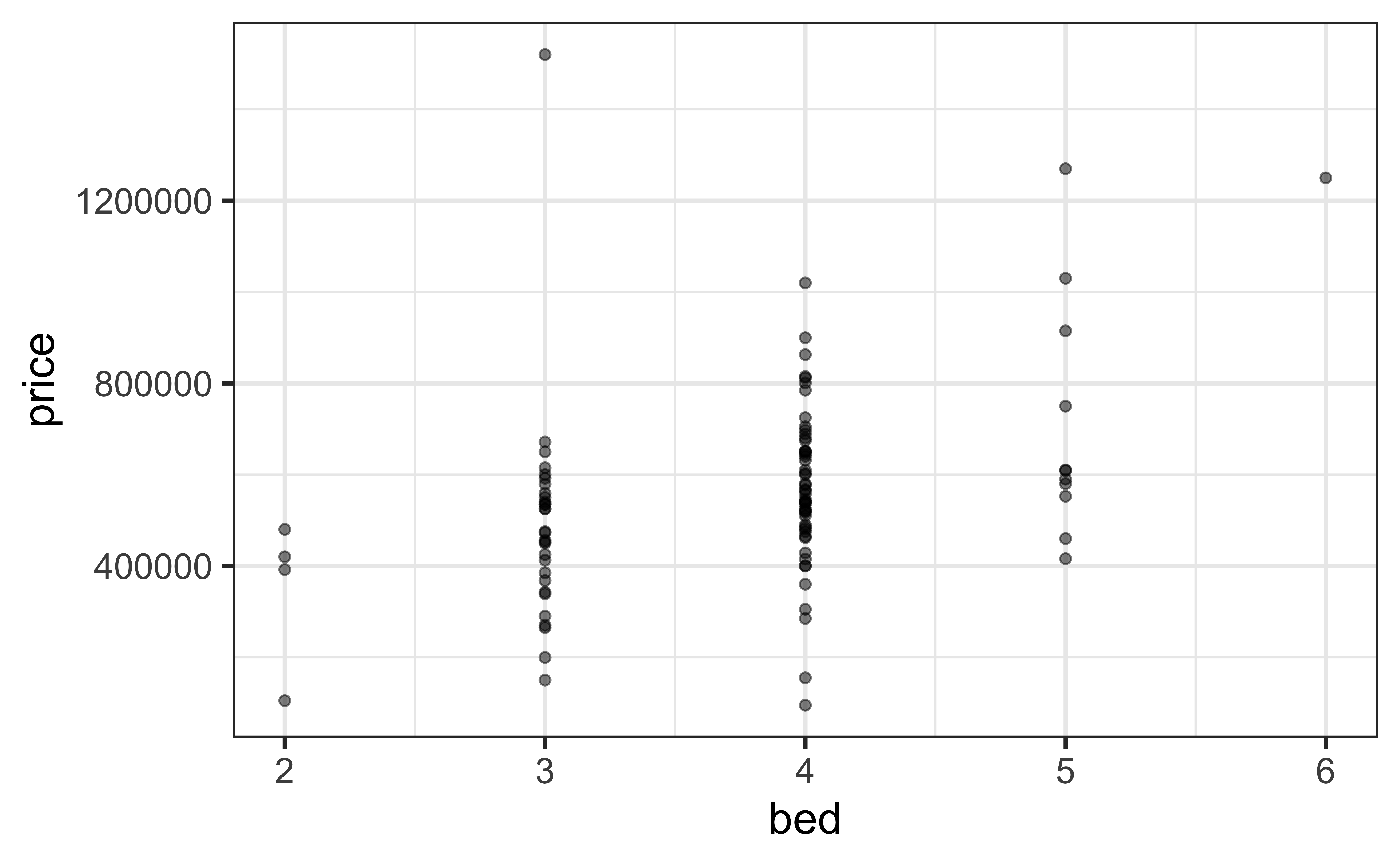
Price vs. bedrooms
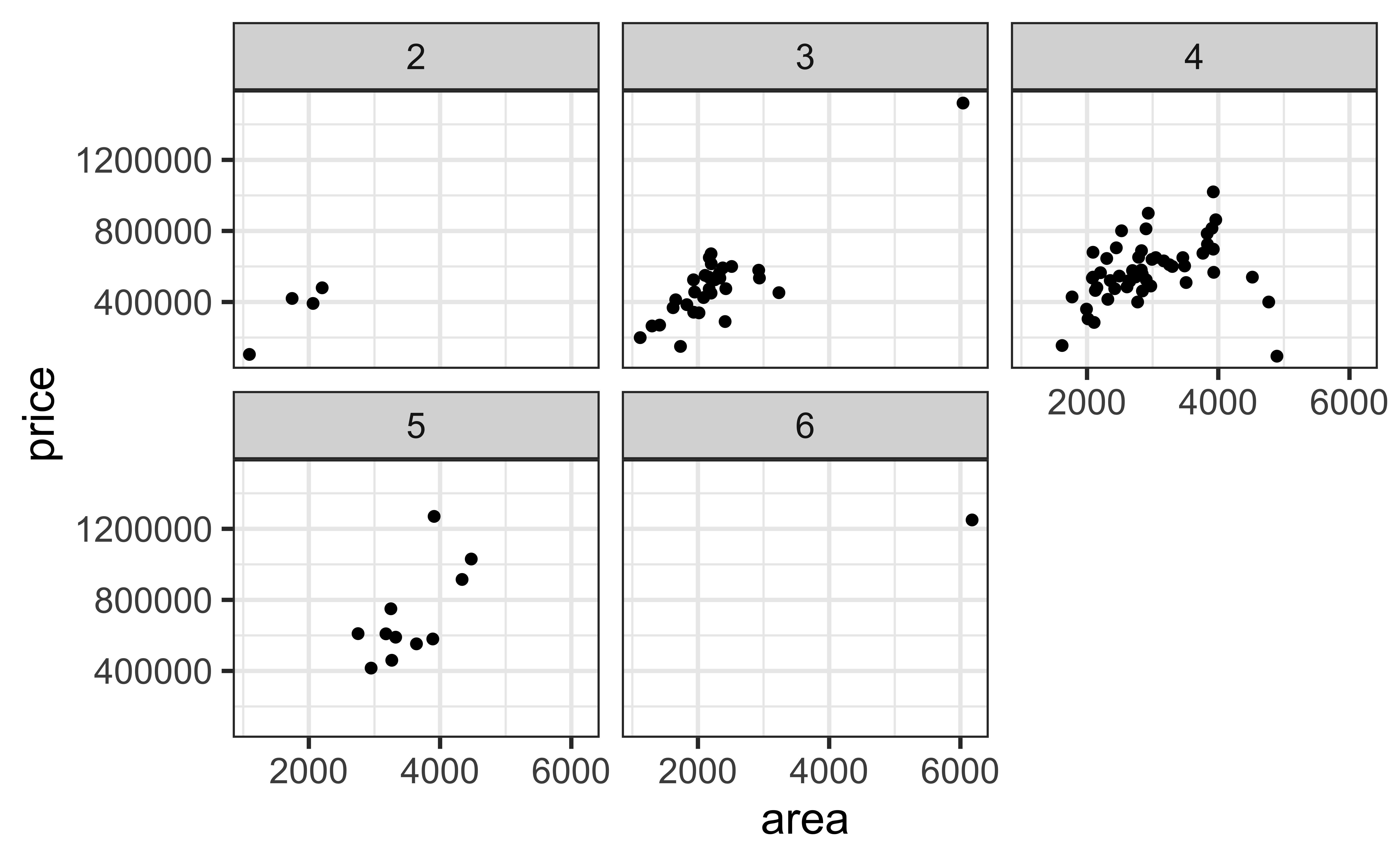
Price vs. area + bedrooms
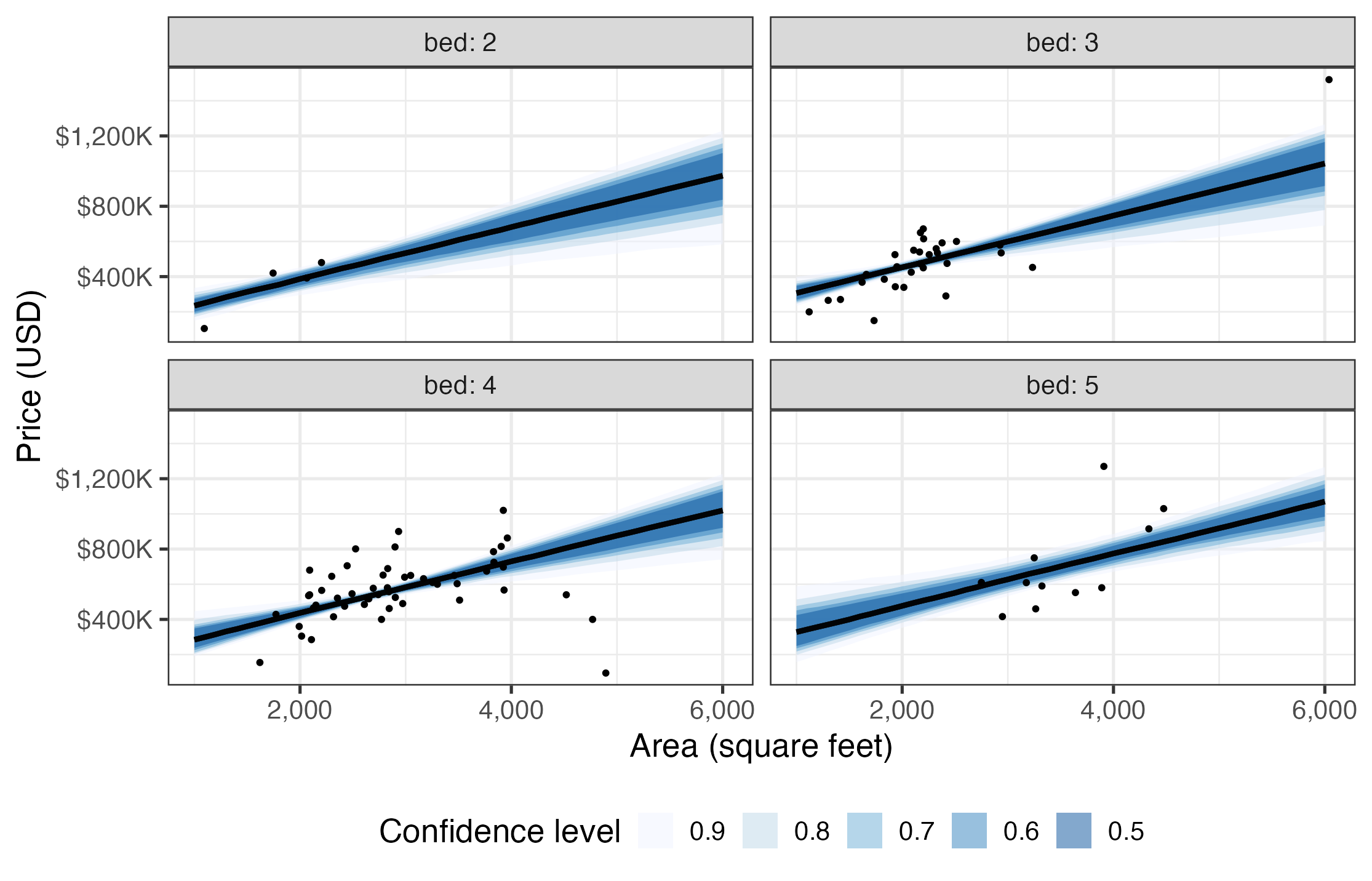
ae-12: Part 1
The following visualization shows bootstrap confidence intervals for predictions from additive (main effects) models for predicting price from area and number of bedrooms. Recreate the visualization. Once you’re done, share your code and plot on Slack in #general.
ae-12: Part 2
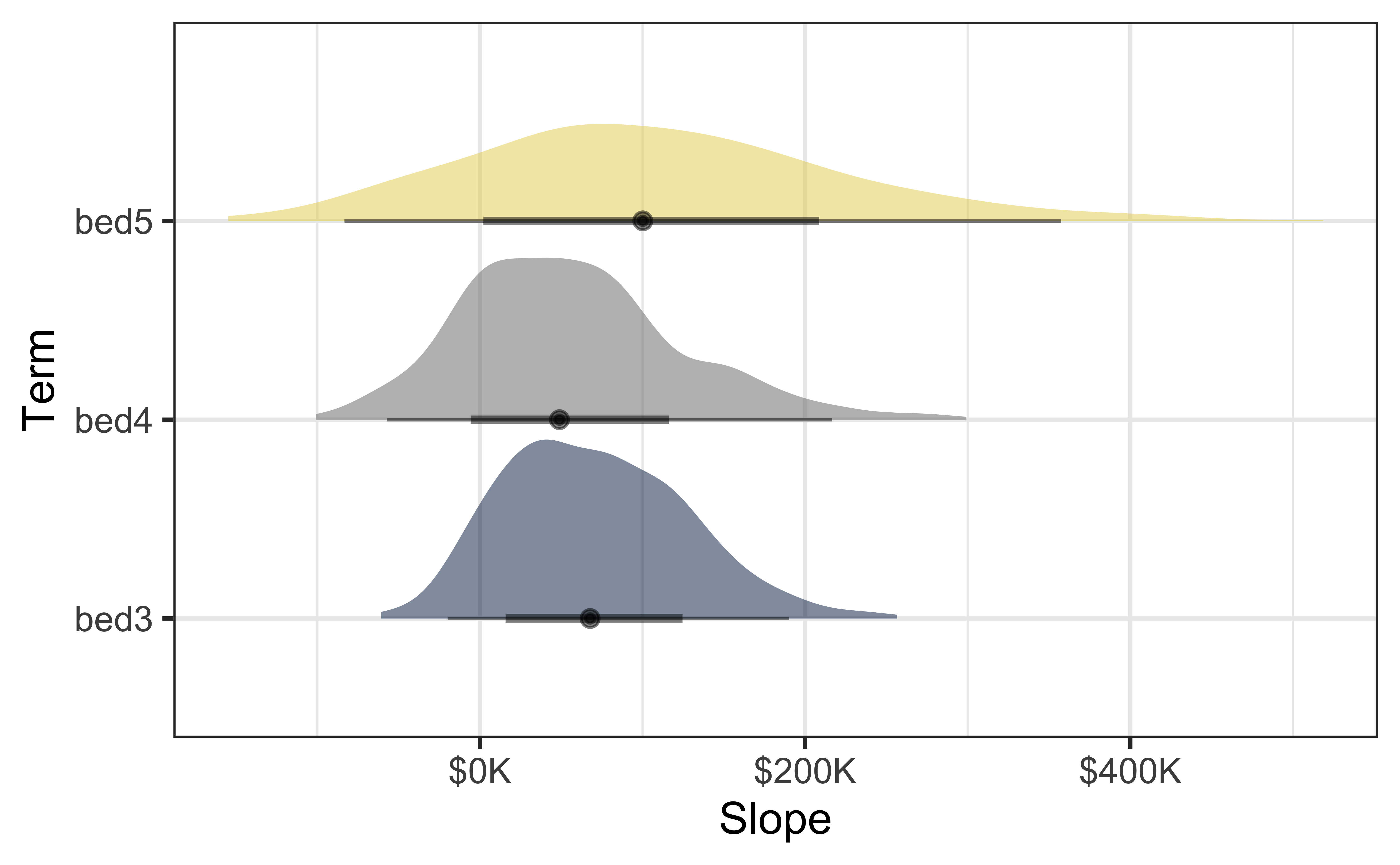
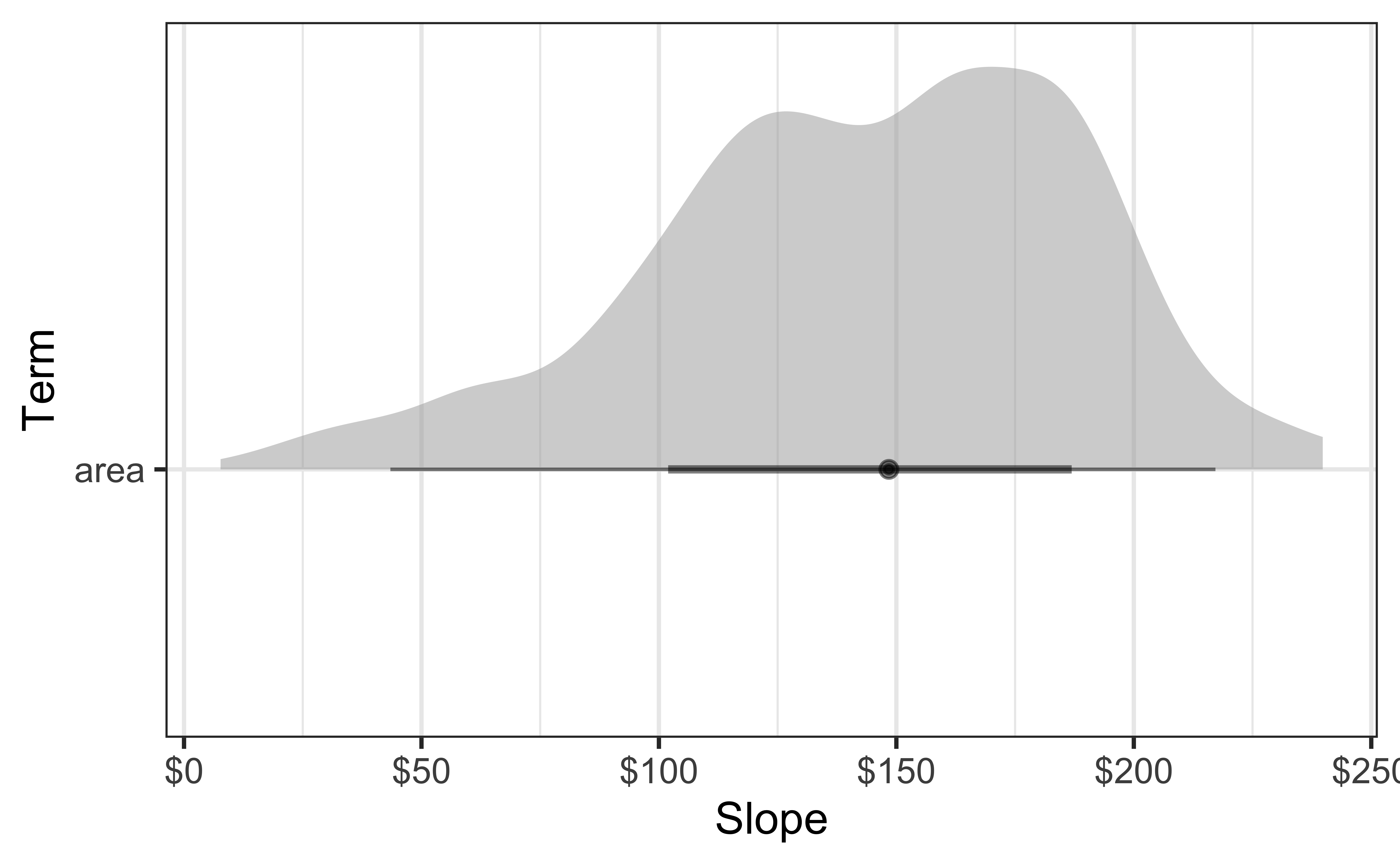
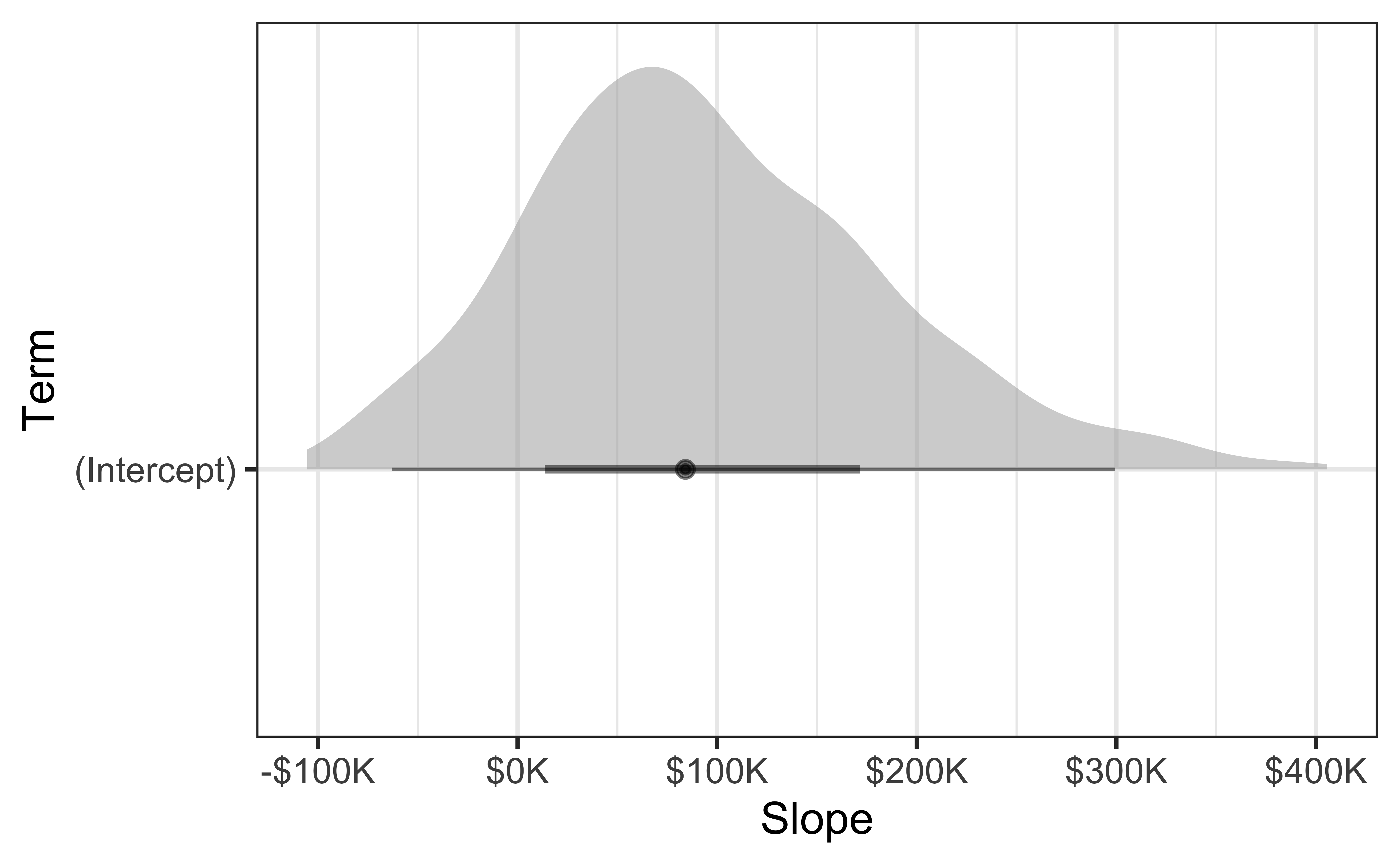
Construct and visualize bootstrap distributions of model estimates using halfeye plots, i.e., recreate the following visualization. Once you’re done, share your code and plot on Slack in #general. Then, try other stats (other ways of visualizing the distributions) from the ggdist package.
![]()