Visualizing geospatial data II

Lecture 17

Dr. Mine Çetinkaya-Rundel

Duke University
STA 313 - Spring 2026

Warm up

Announcements

Please fill out the Project 2 presentation timing survey on Canvas:

https://canvas.duke.edu/courses/71474/assignments/350575

by the end of the day tomorrow (Thursday, March 19)

Setup

# load packages
library(tidyverse)
library(tidyverse)
library(geodata)
library(ggrepel)
library(ggspatial)
library(patchwork)
library(rnaturalearth)
library(rnaturalearthdata)
library(sf)
library(ggnewscale)
library(magick)
library(stars)
library(tmap)

# set theme for ggplot2
ggplot2::theme_set(ggplot2::theme_minimal(base_size = 16))

# set figure parameters for knitr
knitr::opts_chunk$set(
  fig.width = 7, # 7" width
  fig.asp = 0.618, # the golden ratio
  fig.retina = 3, # dpi multiplier for displaying HTML output on retina
  fig.align = "center", # center align figures
  dpi = 300 # higher dpi, sharper image
)

Spatial data in R

Packages for geospatial data in R

R has a rich package ecosystem for read/writing, manipulating, and analyzing geospatial data.

Some core packages:

• sp - core classes for handling spatial data, additional utility functions - Deprecated

• rgdal - R interface to gdal (Geospatial Data Abstraction Library) for reading and writing spatial data - Deprecated

• rgeos - R interface to geos (Geometry Engine Open Source) library for querying and manipulating spatial data. Reading and writing WKT. - Deprecated

• sf - Combines the functionality of sp, rgdal, and rgeos into a single package based on tidy simple features.

• raster - classes and tools for handling spatial raster data.

• stars - Reading, manipulating, writing and plotting spatiotemporal arrays (rasters)

See more - Spatial task view

The sf package

A package that provides simple features access for R:

• represents simple features as records in a data.frame or tibble with a geometry list-column
• represents natively in R all 17 simple feature types for all dimensions

Learn more at r-spatial.github.io/sf.

Installing sf

This is the hardest part of using the sf package, difficulty comes from is dependence on several external libraries (geos, gdal, and proj).

• If using the containers, sf is already installed for you.
• If using your own machine:
  • Windows - installing from source works when Rtools is installed (system requirements are downloaded from rwinlib)
  • MacOS - install dependencies via homebrew: gdal2, geos, proj.
  • Linux - Install development packages for GDAL (>= 2.0.0), GEOS (>= 3.3.0) and Proj.4 (>= 4.8.0) from your package manager of choice.

More specific details are included in the package README on github.

Simple Features for R

Illustration by Allison Horst.

Simple Features

Using sf

Get world data

Using the rnaturalearth package

world <- ne_countries(scale = "medium", returnclass = "sf")
class(world)

[1] "sf"         "data.frame"

What’s in world?

names(world)

  [1] "featurecla" "scalerank"  "labelrank"  "sovereignt" "sov_a3"    
  [6] "adm0_dif"   "level"      "type"       "tlc"        "admin"     
 [11] "adm0_a3"    "geou_dif"   "geounit"    "gu_a3"      "su_dif"    
 [16] "subunit"    "su_a3"      "brk_diff"   "name"       "name_long" 
 [21] "brk_a3"     "brk_name"   "brk_group"  "abbrev"     "postal"    
 [26] "formal_en"  "formal_fr"  "name_ciawf" "note_adm0"  "note_brk"  
 [31] "name_sort"  "name_alt"   "mapcolor7"  "mapcolor8"  "mapcolor9" 
 [36] "mapcolor13" "pop_est"    "pop_rank"   "pop_year"   "gdp_md"    
 [41] "gdp_year"   "economy"    "income_grp" "fips_10"    "iso_a2"    
 [46] "iso_a2_eh"  "iso_a3"     "iso_a3_eh"  "iso_n3"     "iso_n3_eh" 
 [51] "un_a3"      "wb_a2"      "wb_a3"      "woe_id"     "woe_id_eh" 
 [56] "woe_note"   "adm0_iso"   "adm0_diff"  "adm0_tlc"   "adm0_a3_us"
 [61] "adm0_a3_fr" "adm0_a3_ru" "adm0_a3_es" "adm0_a3_cn" "adm0_a3_tw"
 [66] "adm0_a3_in" "adm0_a3_np" "adm0_a3_pk" "adm0_a3_de" "adm0_a3_gb"
 [71] "adm0_a3_br" "adm0_a3_il" "adm0_a3_ps" "adm0_a3_sa" "adm0_a3_eg"
 [76] "adm0_a3_ma" "adm0_a3_pt" "adm0_a3_ar" "adm0_a3_jp" "adm0_a3_ko"
 [81] "adm0_a3_vn" "adm0_a3_tr" "adm0_a3_id" "adm0_a3_pl" "adm0_a3_gr"
 [86] "adm0_a3_it" "adm0_a3_nl" "adm0_a3_se" "adm0_a3_bd" "adm0_a3_ua"
 [91] "adm0_a3_un" "adm0_a3_wb" "continent"  "region_un"  "subregion" 
 [96] "region_wb"  "name_len"   "long_len"   "abbrev_len" "tiny"      
[101] "homepart"   "min_zoom"   "min_label"  "max_label"  "label_x"   
[106] "label_y"    "ne_id"      "wikidataid" "name_ar"    "name_bn"   
[111] "name_de"    "name_en"    "name_es"    "name_fa"    "name_fr"   
[116] "name_el"    "name_he"    "name_hi"    "name_hu"    "name_id"   
[121] "name_it"    "name_ja"    "name_ko"    "name_nl"    "name_pl"   
[126] "name_pt"    "name_ru"    "name_sv"    "name_tr"    "name_uk"   
[131] "name_ur"    "name_vi"    "name_zh"    "name_zht"   "fclass_iso"
[136] "tlc_diff"   "fclass_tlc" "fclass_us"  "fclass_fr"  "fclass_ru" 
[141] "fclass_es"  "fclass_cn"  "fclass_tw"  "fclass_in"  "fclass_np" 
[146] "fclass_pk"  "fclass_de"  "fclass_gb"  "fclass_br"  "fclass_il" 
[151] "fclass_ps"  "fclass_sa"  "fclass_eg"  "fclass_ma"  "fclass_pt" 
[156] "fclass_ar"  "fclass_jp"  "fclass_ko"  "fclass_vn"  "fclass_tr" 
[161] "fclass_id"  "fclass_pl"  "fclass_gr"  "fclass_it"  "fclass_nl" 
[166] "fclass_se"  "fclass_bd"  "fclass_ua"  "geometry"  

What’s in world?

attributes(world)

$names
  [1] "featurecla" "scalerank"  "labelrank"  "sovereignt" "sov_a3"    
  [6] "adm0_dif"   "level"      "type"       "tlc"        "admin"     
 [11] "adm0_a3"    "geou_dif"   "geounit"    "gu_a3"      "su_dif"    
 [16] "subunit"    "su_a3"      "brk_diff"   "name"       "name_long" 
 [21] "brk_a3"     "brk_name"   "brk_group"  "abbrev"     "postal"    
 [26] "formal_en"  "formal_fr"  "name_ciawf" "note_adm0"  "note_brk"  
 [31] "name_sort"  "name_alt"   "mapcolor7"  "mapcolor8"  "mapcolor9" 
 [36] "mapcolor13" "pop_est"    "pop_rank"   "pop_year"   "gdp_md"    
 [41] "gdp_year"   "economy"    "income_grp" "fips_10"    "iso_a2"    
 [46] "iso_a2_eh"  "iso_a3"     "iso_a3_eh"  "iso_n3"     "iso_n3_eh" 
 [51] "un_a3"      "wb_a2"      "wb_a3"      "woe_id"     "woe_id_eh" 
 [56] "woe_note"   "adm0_iso"   "adm0_diff"  "adm0_tlc"   "adm0_a3_us"
 [61] "adm0_a3_fr" "adm0_a3_ru" "adm0_a3_es" "adm0_a3_cn" "adm0_a3_tw"
 [66] "adm0_a3_in" "adm0_a3_np" "adm0_a3_pk" "adm0_a3_de" "adm0_a3_gb"
 [71] "adm0_a3_br" "adm0_a3_il" "adm0_a3_ps" "adm0_a3_sa" "adm0_a3_eg"
 [76] "adm0_a3_ma" "adm0_a3_pt" "adm0_a3_ar" "adm0_a3_jp" "adm0_a3_ko"
 [81] "adm0_a3_vn" "adm0_a3_tr" "adm0_a3_id" "adm0_a3_pl" "adm0_a3_gr"
 [86] "adm0_a3_it" "adm0_a3_nl" "adm0_a3_se" "adm0_a3_bd" "adm0_a3_ua"
 [91] "adm0_a3_un" "adm0_a3_wb" "continent"  "region_un"  "subregion" 
 [96] "region_wb"  "name_len"   "long_len"   "abbrev_len" "tiny"      
[101] "homepart"   "min_zoom"   "min_label"  "max_label"  "label_x"   
[106] "label_y"    "ne_id"      "wikidataid" "name_ar"    "name_bn"   
[111] "name_de"    "name_en"    "name_es"    "name_fa"    "name_fr"   
[116] "name_el"    "name_he"    "name_hi"    "name_hu"    "name_id"   
[121] "name_it"    "name_ja"    "name_ko"    "name_nl"    "name_pl"   
[126] "name_pt"    "name_ru"    "name_sv"    "name_tr"    "name_uk"   
[131] "name_ur"    "name_vi"    "name_zh"    "name_zht"   "fclass_iso"
[136] "tlc_diff"   "fclass_tlc" "fclass_us"  "fclass_fr"  "fclass_ru" 
[141] "fclass_es"  "fclass_cn"  "fclass_tw"  "fclass_in"  "fclass_np" 
[146] "fclass_pk"  "fclass_de"  "fclass_gb"  "fclass_br"  "fclass_il" 
[151] "fclass_ps"  "fclass_sa"  "fclass_eg"  "fclass_ma"  "fclass_pt" 
[156] "fclass_ar"  "fclass_jp"  "fclass_ko"  "fclass_vn"  "fclass_tr" 
[161] "fclass_id"  "fclass_pl"  "fclass_gr"  "fclass_it"  "fclass_nl" 
[166] "fclass_se"  "fclass_bd"  "fclass_ua"  "geometry"  

$sf_column
[1] "geometry"

$agr
featurecla  scalerank       <NA>       <NA>       <NA>       <NA>       <NA> 
      <NA>       <NA>       <NA>       <NA>       <NA>       <NA>       <NA> 
      <NA>       <NA>       <NA>       <NA>       <NA>       <NA>       <NA> 
      <NA>       <NA>       <NA>       <NA>       <NA>       <NA>       <NA> 
      <NA>       <NA>       <NA>       <NA>       <NA>       <NA>       <NA> 
      <NA>       <NA>       <NA>       <NA>       <NA>       <NA>       <NA> 
      <NA>       <NA>       <NA>       <NA>       <NA>       <NA>       <NA> 
      <NA>       <NA>       <NA>       <NA>       <NA>       <NA>       <NA> 
      <NA>       <NA>       <NA>       <NA>       <NA>       <NA>       <NA> 
      <NA>       <NA>       <NA>       <NA>       <NA>       <NA>       <NA> 
      <NA>       <NA>       <NA>       <NA>       <NA>       <NA>       <NA> 
      <NA>       <NA>       <NA>       <NA>       <NA>       <NA>       <NA> 
      <NA>       <NA>       <NA>       <NA>       <NA>       <NA>       <NA> 
      <NA>       <NA>       <NA>       <NA>       <NA>       <NA>       <NA> 
      <NA>       <NA>       <NA>       <NA>       <NA>       <NA>       <NA> 
      <NA>       <NA>       <NA>       <NA>       <NA>       <NA>       <NA> 
      <NA>       <NA>       <NA>       <NA>       <NA>       <NA>       <NA> 
      <NA>       <NA>       <NA>       <NA>       <NA>       <NA>       <NA> 
      <NA>       <NA>       <NA>       <NA>       <NA>       <NA>       <NA> 
      <NA>       <NA>       <NA>       <NA>       <NA>       <NA>       <NA> 
      <NA>       <NA>       <NA>       <NA>       <NA>       <NA>       <NA> 
      <NA>       <NA>       <NA>       <NA>       <NA>       <NA>       <NA> 
      <NA>       <NA>       <NA>       <NA>       <NA>       <NA>       <NA> 
      <NA>       <NA>       <NA>       <NA>       <NA>       <NA>       <NA> 
      <NA>       <NA>       <NA>       <NA>       <NA>       <NA>       <NA> 
      <NA>       <NA>       <NA>       <NA>       <NA>       <NA>       <NA> 
      <NA>       <NA>       <NA>       <NA>       <NA>       <NA>       <NA> 
      <NA>       <NA>       <NA>       <NA>       <NA>       <NA>       <NA> 
      <NA>       <NA>       <NA>       <NA>       <NA>       <NA>       <NA> 
      <NA>       <NA>       <NA>       <NA>       <NA>       <NA>       <NA> 
      <NA>       <NA>       <NA>       <NA>       <NA>       <NA>       <NA> 
      <NA>       <NA>       <NA>       <NA>       <NA>       <NA>       <NA> 
      <NA>       <NA>       <NA>       <NA>       <NA>       <NA>       <NA> 
      <NA>       <NA>       <NA>       <NA>       <NA>       <NA>       <NA> 
      <NA>       <NA>       <NA>       <NA>       <NA>       <NA>       <NA> 
      <NA>       <NA>       <NA>       <NA>       <NA>       <NA>       <NA> 
      <NA>       <NA>       <NA>       <NA>       <NA>       <NA>       <NA> 
      <NA>       <NA>       <NA>       <NA>       <NA>       <NA>       <NA> 
      <NA>       <NA>       <NA>       <NA>       <NA>       <NA>       <NA> 
      <NA>       <NA>       <NA>       <NA>       <NA>       <NA>       <NA> 
      <NA>       <NA>       <NA>       <NA>       <NA>       <NA>       <NA> 
      <NA>       <NA>       <NA>       <NA>       <NA>       <NA>       <NA> 
      <NA>       <NA>       <NA>       <NA>       <NA>       <NA>       <NA> 
      <NA>       <NA>       <NA>       <NA>       <NA>       <NA>       <NA> 
      <NA>       <NA>       <NA>       <NA>       <NA>       <NA>       <NA> 
      <NA>       <NA>       <NA>       <NA>       <NA>       <NA>       <NA> 
      <NA>       <NA>       <NA>       <NA>       <NA>       <NA>       <NA> 
      <NA>       <NA>       <NA>       <NA>       <NA>       <NA>       <NA> 
Levels: constant aggregate identity

$row.names
  [1]   1   2   3   4   5   6   7   8   9  10  11  12  13  14  15  16  17  18
 [19]  19  20  21  22  23  24  25  26  27  28  29  30  31  32  33  34  35  36
 [37]  37  38  39  40  41  42  43  44  45  46  47  48  49  50  51  52  53  54
 [55]  55  56  57  58  59  60  61  62  63  64  65  66  67  68  69  70  71  72
 [73]  73  74  75  76  77  78  79  80  81  82  83  84  85  86  87  88  89  90
 [91]  91  92  93  94  95  96  97  98  99 100 101 102 103 104 105 106 107 108
[109] 109 110 111 112 113 114 115 116 117 118 119 120 121 122 123 124 125 126
[127] 127 128 129 130 131 132 133 134 135 136 137 138 139 140 141 142 143 144
[145] 145 146 147 148 149 150 151 152 153 154 155 156 157 158 159 160 161 162
[163] 163 164 165 166 167 168 169 170 171 172 173 174 175 176 177 178 179 180
[181] 181 182 183 184 185 186 187 188 189 190 191 192 193 194 195 196 197 198
[199] 199 200 201 202 203 204 205 206 207 208 209 210 211 212 213 214 215 216
[217] 217 218 219 220 221 222 223 224 225 226 227 228 229 230 231 232 233 234
[235] 235 236 237 238 239 240 241 242

$class
[1] "sf"         "data.frame"

sf geometry

world |>
  select(geometry)

Simple feature collection with 242 features and 0 fields
Geometry type: MULTIPOLYGON
Dimension:     XY
Bounding box:  xmin: -180 ymin: -89.99893 xmax: 180 ymax: 83.59961
Geodetic CRS:  WGS 84
First 10 features:
                         geometry
1  MULTIPOLYGON (((31.28789 -2...
2  MULTIPOLYGON (((30.39609 -1...
3  MULTIPOLYGON (((53.08564 16...
4  MULTIPOLYGON (((104.064 10....
5  MULTIPOLYGON (((-60.82119 9...
6  MULTIPOLYGON (((12.43916 41...
7  MULTIPOLYGON (((166.7458 -1...
8  MULTIPOLYGON (((70.94678 42...
9  MULTIPOLYGON (((-53.37061 -...
10 MULTIPOLYGON (((162.9832 5....

Map the world with sf

ggplot(data = world) +
  geom_sf()

Plays nicely with ggplot2

ggplot(data = world) +
  geom_sf(fill = "cornsilk", size = 0.2) +
  labs(x = "Longitude", y = "Latitude", title = "World map") +
  theme(panel.background = element_rect("lightblue"))

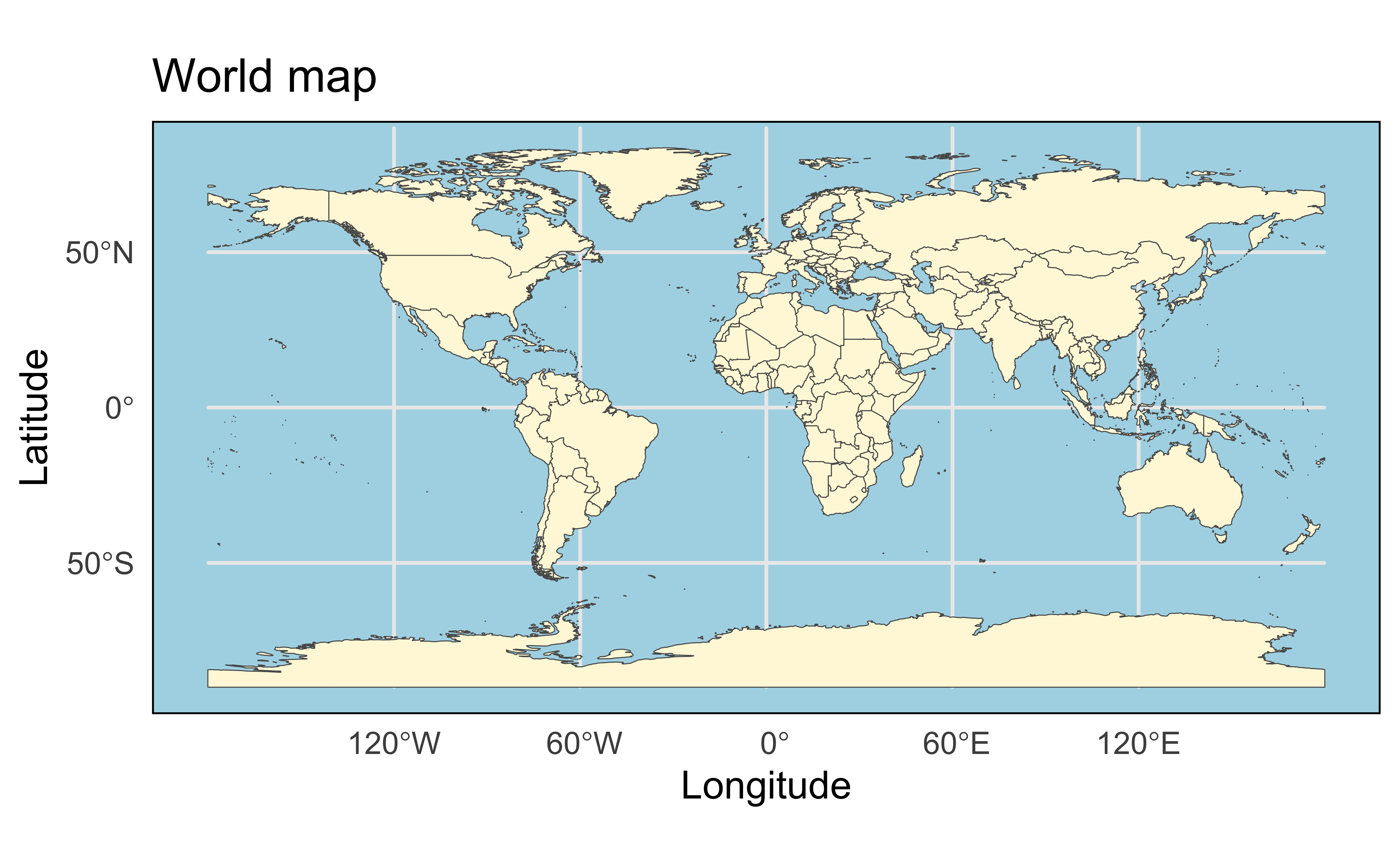
Plays nicely with ggplot2

ggplot(data = world) +
  geom_sf(aes(fill = pop_est)) +
  scale_fill_viridis_c(option = "plasma", trans = "sqrt")

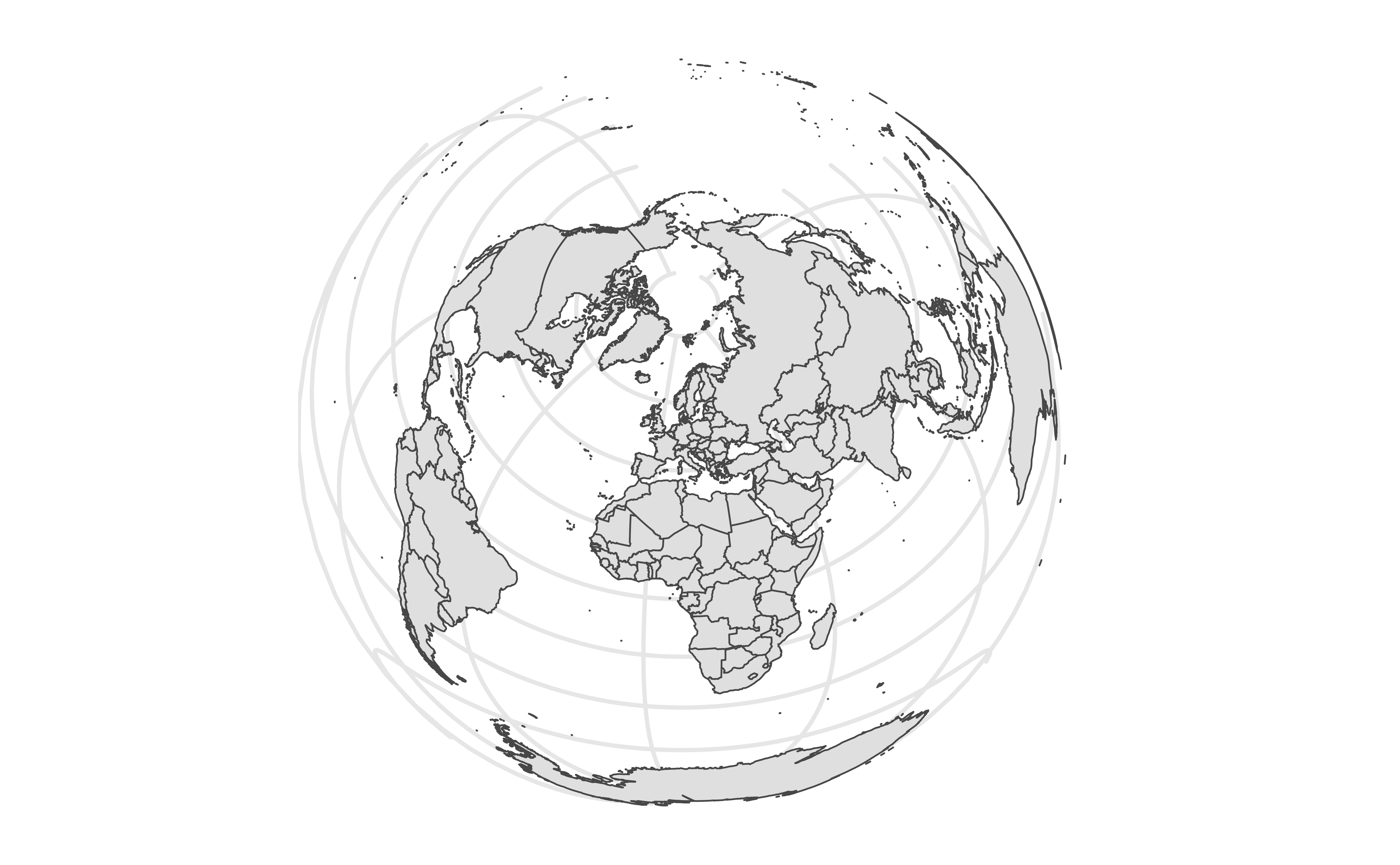
Projections with sf

ggplot(data = world) +
  geom_sf() +
  coord_sf(
    crs = "+proj=laea +lat_0=52 +lon_0=10 +x_0=4321000 +y_0=3210000 +ellps=GRS80 +units=m +no_defs"
  )

Scale bar and North arrow

Using the ggspatial package:

ggplot(data = world) +
  geom_sf(fill = "cornsilk") +
  annotation_scale(location = "bl", width_hint = 0.4) +
  annotation_north_arrow(
    location = "bl",
    which_north = "true",
    pad_x = unit(0.5, "in"),
    pad_y = unit(0.3, "in"),
    style = north_arrow_fancy_orienteering
  ) +
  coord_sf(xlim = c(24, 45), ylim = c(32, 43))

Scale bar and North arrow

Scale on map varies by more than 10%, scale bar may be inaccurate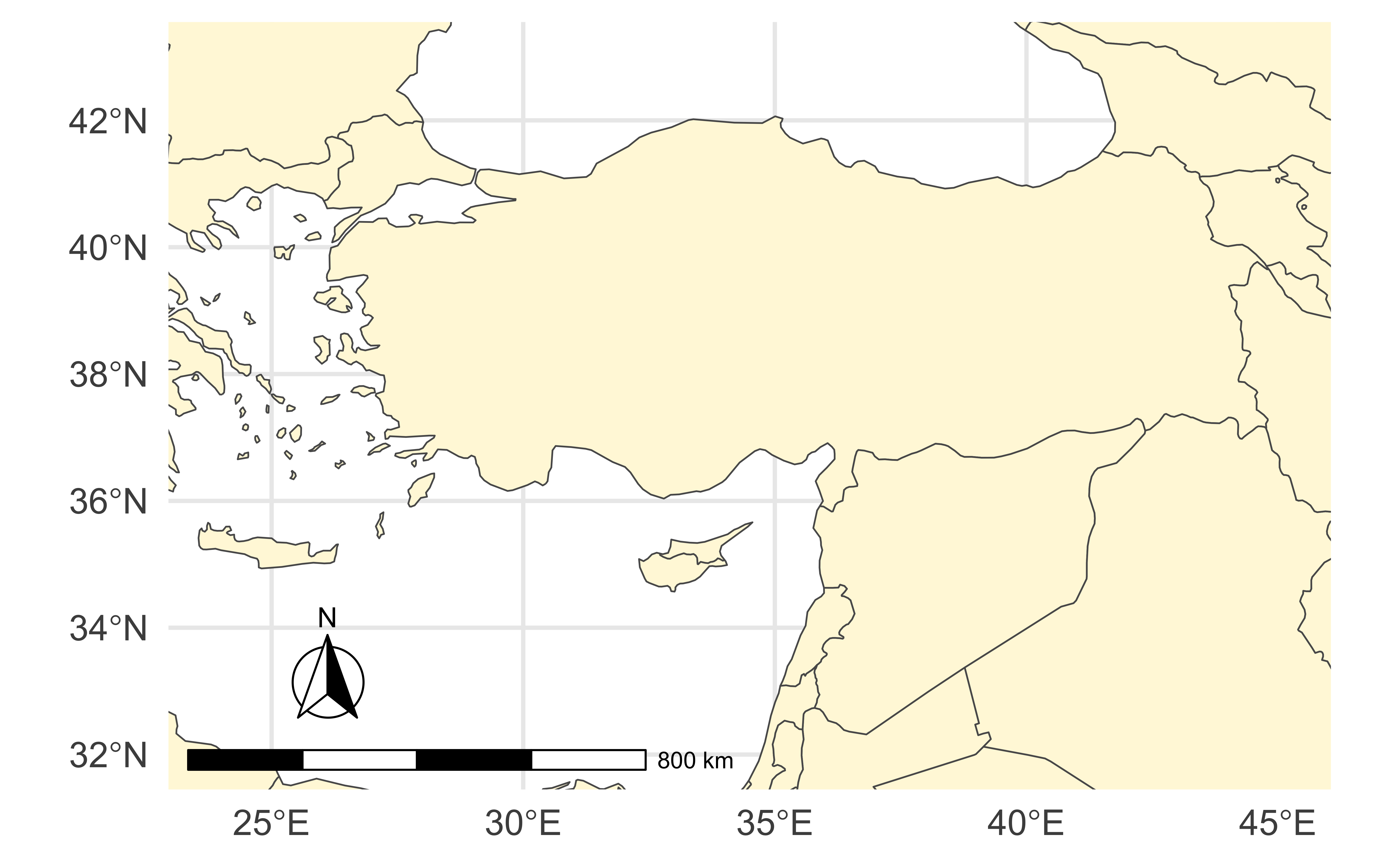

The scale warning

Scale on map varies by more than 10%, scale bar may be inaccurate

Note the warning of the inaccurate scale bar: since the map uses unprojected data in longitude/latitude (WGS84) on an equidistant cylindrical projection (all meridians being parallel), length in (kilo)meters on the map directly depends mathematically on the degree of latitude. Plots of small regions or projected data will often allow for more accurate scale bars.

Source: Drawing beautiful maps programmatically with R, sf and ggplot2 — Part 1: Basics

Reading, writing, and converting

• sf
  • st_read() / st_write() - Shapefile, GeoJSON, KML, …
  • read_sf() / write_sf() - Same, supports tibbles …
  • st_as_sfc() / st_as_wkt() - sf <-> WKT
  • st_as_sfc() / st_as_binary() - sf <-> WKB
  • st_as_sfc() / as(x, "Spatial") - sf <-> sp

See sf vignette #2 - Reading, Writing and Converting Simple Features.

Example data

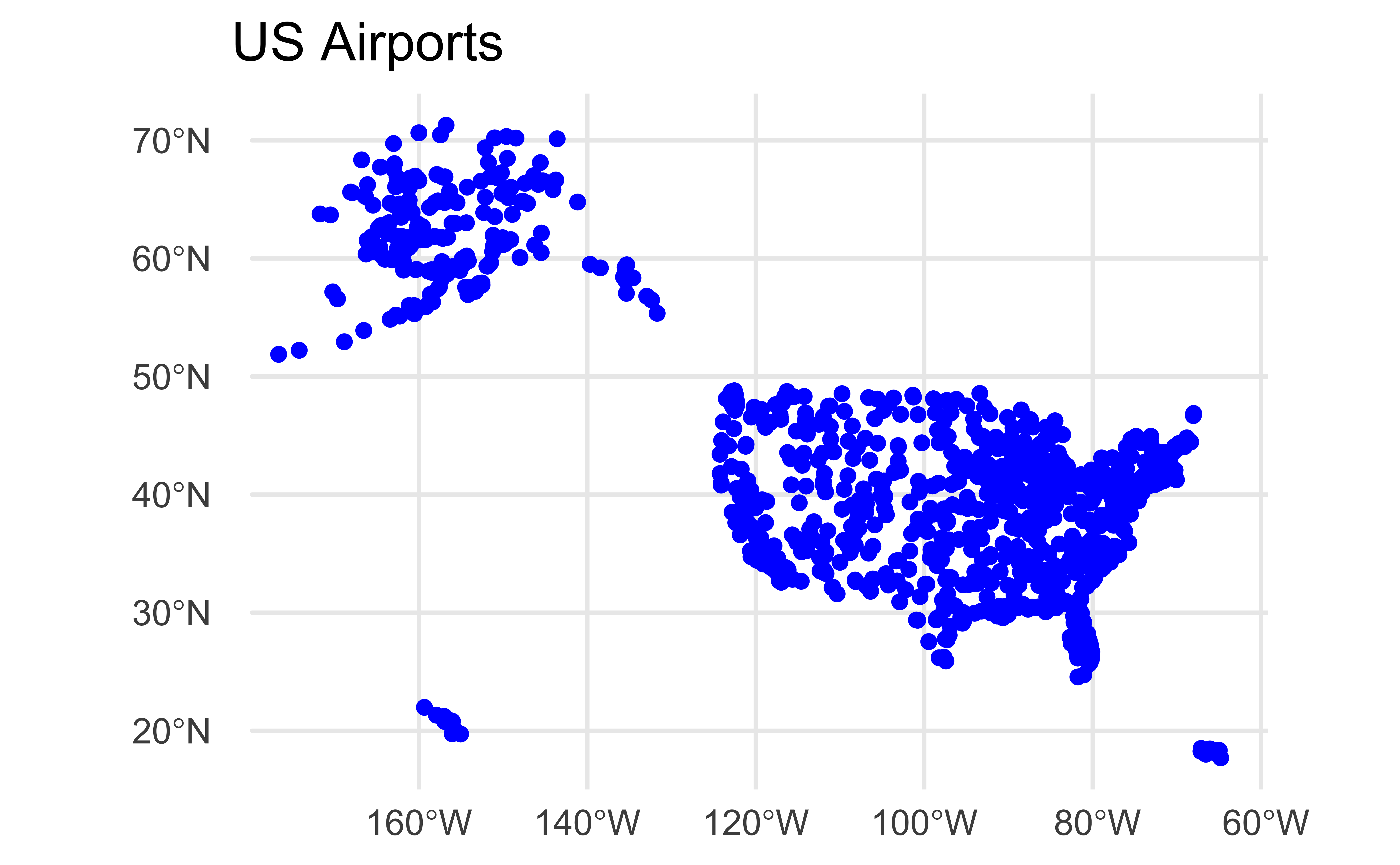
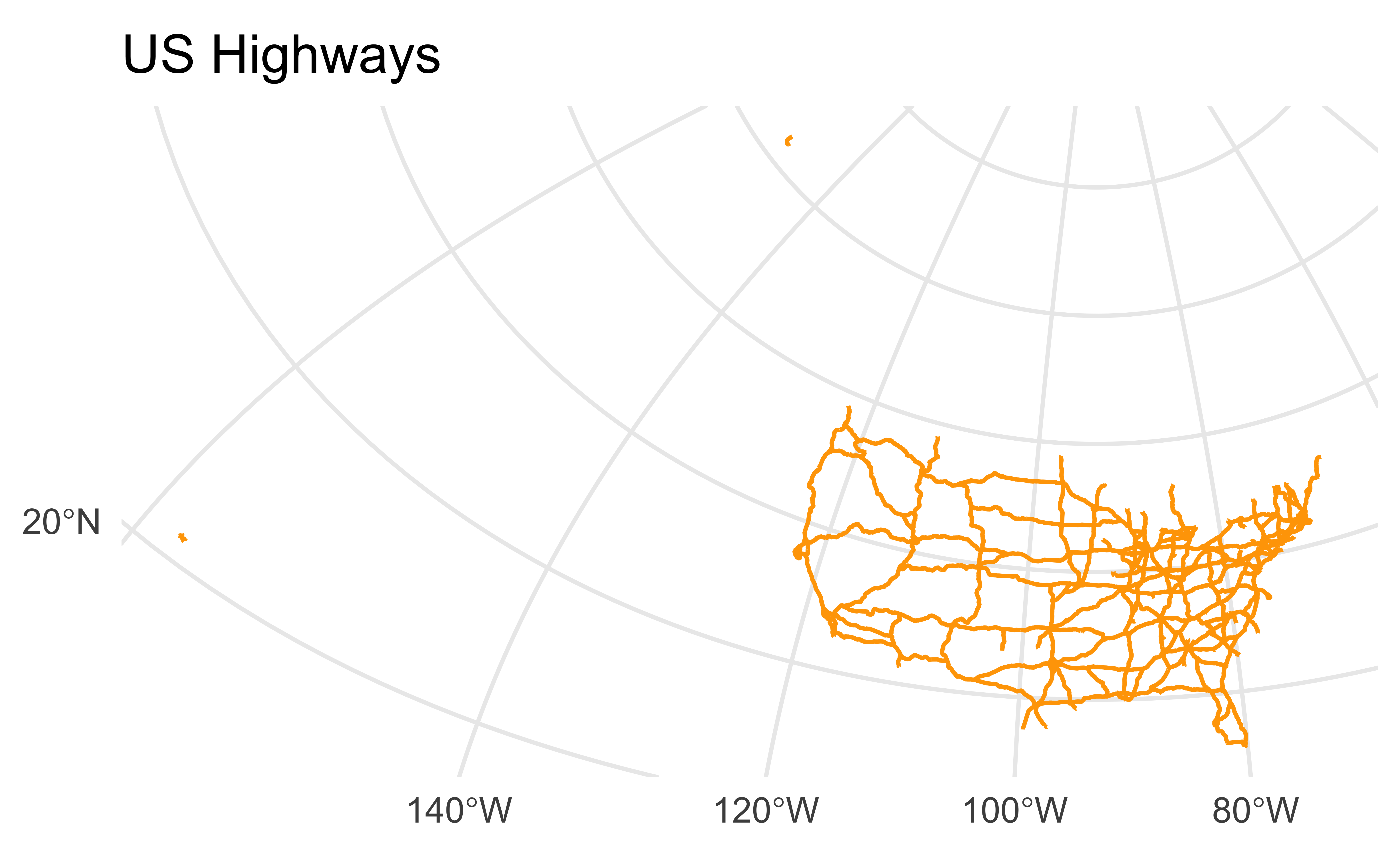
North Carolina counties, US airports, and US highways:

nc <- read_sf("data/nc_counties/", quiet = TRUE)
air <- read_sf("data/airports/", quiet = TRUE)
hwy <- read_sf("data/us_interstates/", quiet = TRUE)

NC Counties

nc

Simple feature collection with 100 features and 8 fields
Geometry type: MULTIPOLYGON
Dimension:     XY
Bounding box:  xmin: -84.32186 ymin: 33.84175 xmax: -75.46003 ymax: 36.58815
Geodetic CRS:  NAD83
# A tibble: 100 × 9
     AREA PERIMETER COUNTYP010 STATE COUNTY          FIPS  STATE_FIPS SQUARE_MIL
    <dbl>     <dbl>      <dbl> <chr> <chr>           <chr> <chr>           <dbl>
 1 0.112       1.61       1994 NC    Ashe County     37009 37               429.
 2 0.0616      1.35       1996 NC    Alleghany Coun… 37005 37               236.
 3 0.140       1.77       1998 NC    Surry County    37171 37               539.
 4 0.0891      1.43       1999 NC    Gates County    37073 37               342.
 5 0.0687      4.43       2000 NC    Currituck Coun… 37053 37               264.
 6 0.119       1.40       2001 NC    Stokes County   37169 37               456.
 7 0.0626      2.11       2002 NC    Camden County   37029 37               241.
 8 0.115       1.46       2003 NC    Warren County   37185 37               444.
 9 0.143       2.40       2004 NC    Northampton Co… 37131 37               551.
10 0.0925      1.81       2005 NC    Hertford County 37091 37               356.
# ℹ 90 more rows
# ℹ 1 more variable: geometry <MULTIPOLYGON [°]>

US Airports

air

Simple feature collection with 940 features and 16 fields
Geometry type: POINT
Dimension:     XY
Bounding box:  xmin: -176.646 ymin: 17.70156 xmax: -64.80172 ymax: 71.28545
Geodetic CRS:  NAD83
# A tibble: 940 × 17
   AIRPRTX010 FEATURE ICAO  IATA  AIRPT_NAME CITY  STATE STATE_FIPS COUNTY FIPS 
        <dbl> <chr>   <chr> <chr> <chr>      <chr> <chr> <chr>      <chr>  <chr>
 1          0 AIRPORT KGON  GON   GROTON-NE… GROT… CT    09         NEW L… 09011
 2          3 AIRPORT K6S5  6S5   RAVALLI C… HAMI… MT    30         RAVAL… 30081
 3          4 AIRPORT KMHV  MHV   MOJAVE AI… MOJA… CA    06         KERN   06029
 4          6 AIRPORT KSEE  SEE   GILLESPIE… SAN … CA    06         SAN D… 06073
 5          7 AIRPORT KFPR  FPR   ST LUCIE … FORT… FL    12         ST LU… 12111
 6          8 AIRPORT KRYY  RYY   COBB COUN… ATLA… GA    13         COBB   13067
 7         10 AIRPORT KMKL  MKL   MC KELLAR… JACK… TN    47         MADIS… 47113
 8         11 AIRPORT KCCR  CCR   BUCHANAN … CONC… CA    06         CONTR… 06013
 9         13 AIRPORT KJYO  JYO   LEESBURG … LEES… VA    51         LOUDO… 51107
10         15 AIRPORT KCAD  CAD   WEXFORD C… CADI… MI    26         WEXFO… 26165
# ℹ 930 more rows
# ℹ 7 more variables: TOT_ENP <dbl>, LATITUDE <dbl>, LONGITUDE <dbl>,
#   ELEV <dbl>, ACT_DATE <chr>, CNTL_TWR <chr>, geometry <POINT [°]>

US highways

hwy

Simple feature collection with 233 features and 3 fields
Geometry type: MULTILINESTRING
Dimension:     XY
Bounding box:  xmin: -7472582 ymin: 2911107 xmax: 2443707 ymax: 8208428
Projected CRS: NAD83 / UTM zone 15N
# A tibble: 233 × 4
   ROUTE_NUM DIST_MILES DIST_KM                                         geometry
   <chr>          <dbl>   <dbl>                            <MULTILINESTRING [m]>
 1 I10          2449.   3941.   ((-1881200 4072307, -1879922 4072943, -1877750 …
 2 I105           20.8    33.4  ((-1910156 5339585, -1910139 5339705, -1909706 …
 3 I110           41.4    66.6  ((1054139 3388879, 1054287 3385988, 1054967 338…
 4 I115            1.58    2.55 ((-1013796 5284243, -1013138 5283839, -1012546 …
 5 I12            85.3   137.   ((680741.7 3366581, 682709.8 3366521, 683440.5 …
 6 I124            1.73    2.79 ((1201467 3906285, 1201643 3905927, 1201658 390…
 7 I126            3.56    5.72 ((1601502 3829718, 1602136 3829053, 1602406 382…
 8 I129            3.1     4.99 ((217446 4705389, 217835.1 4705377, 219243.7 47…
 9 I135           96.3   155.   ((96922.97 4313125, 96561.85 4310056, 96655.33 …
10 I15          1436.   2311    ((-882875.7 5602902, -882998.3 5602422, -883277…
# ℹ 223 more rows

sf structure

str(nc)

sf [100 × 9] (S3: sf/tbl_df/tbl/data.frame)
 $ AREA      : num [1:100] 0.1118 0.0616 0.1402 0.0891 0.0687 ...
 $ PERIMETER : num [1:100] 1.61 1.35 1.77 1.43 4.43 ...
 $ COUNTYP010: num [1:100] 1994 1996 1998 1999 2000 ...
 $ STATE     : chr [1:100] "NC" "NC" "NC" "NC" ...
 $ COUNTY    : chr [1:100] "Ashe County" "Alleghany County" "Surry County" "Gates County" ...
 $ FIPS      : chr [1:100] "37009" "37005" "37171" "37073" ...
 $ STATE_FIPS: chr [1:100] "37" "37" "37" "37" ...
 $ SQUARE_MIL: num [1:100] 429 236 539 342 264 ...
 $ geometry  :sfc_MULTIPOLYGON of length 100; first list element: List of 1
  ..$ :List of 1
  .. ..$ : num [1:1030, 1:2] -81.7 -81.7 -81.7 -81.6 -81.6 ...
  ..- attr(*, "class")= chr [1:3] "XY" "MULTIPOLYGON" "sfg"
 - attr(*, "sf_column")= chr "geometry"
 - attr(*, "agr")= Factor w/ 3 levels "constant","aggregate",..: NA NA NA NA NA NA NA NA
  ..- attr(*, "names")= chr [1:8] "AREA" "PERIMETER" "COUNTYP010" "STATE" ...

sf classes

class(nc)

[1] "sf"         "tbl_df"     "tbl"        "data.frame"

class(nc$geometry)

[1] "sfc_MULTIPOLYGON" "sfc"             

class(st_geometry(nc))

[1] "sfc_MULTIPOLYGON" "sfc"             

class(nc$geometry[[1]])

[1] "XY"           "MULTIPOLYGON" "sfg"         

Projections / CRS

st_crs(nc)

Coordinate Reference System:
  User input: NAD83 
  wkt:
GEOGCRS["NAD83",
    DATUM["North American Datum 1983",
        ELLIPSOID["GRS 1980",6378137,298.257222101,
            LENGTHUNIT["metre",1]]],
    PRIMEM["Greenwich",0,
        ANGLEUNIT["degree",0.0174532925199433]],
    CS[ellipsoidal,2],
        AXIS["latitude",north,
            ORDER[1],
            ANGLEUNIT["degree",0.0174532925199433]],
        AXIS["longitude",east,
            ORDER[2],
            ANGLEUNIT["degree",0.0174532925199433]],
    ID["EPSG",4269]]

EPSG Geodetic Parameter Dataset

st_crs(hwy)

Coordinate Reference System:
  User input: NAD83 / UTM zone 15N 
  wkt:
PROJCRS["NAD83 / UTM zone 15N",
    BASEGEOGCRS["NAD83",
        DATUM["North American Datum 1983",
            ELLIPSOID["GRS 1980",6378137,298.257222101,
                LENGTHUNIT["metre",1]]],
        PRIMEM["Greenwich",0,
            ANGLEUNIT["degree",0.0174532925199433]],
        ID["EPSG",4269]],
    CONVERSION["UTM zone 15N",
        METHOD["Transverse Mercator",
            ID["EPSG",9807]],
        PARAMETER["Latitude of natural origin",0,
            ANGLEUNIT["Degree",0.0174532925199433],
            ID["EPSG",8801]],
        PARAMETER["Longitude of natural origin",-93,
            ANGLEUNIT["Degree",0.0174532925199433],
            ID["EPSG",8802]],
        PARAMETER["Scale factor at natural origin",0.9996,
            SCALEUNIT["unity",1],
            ID["EPSG",8805]],
        PARAMETER["False easting",500000,
            LENGTHUNIT["metre",1],
            ID["EPSG",8806]],
        PARAMETER["False northing",0,
            LENGTHUNIT["metre",1],
            ID["EPSG",8807]]],
    CS[Cartesian,2],
        AXIS["(E)",east,
            ORDER[1],
            LENGTHUNIT["metre",1]],
        AXIS["(N)",north,
            ORDER[2],
            LENGTHUNIT["metre",1]],
    ID["EPSG",26915]]

Projections

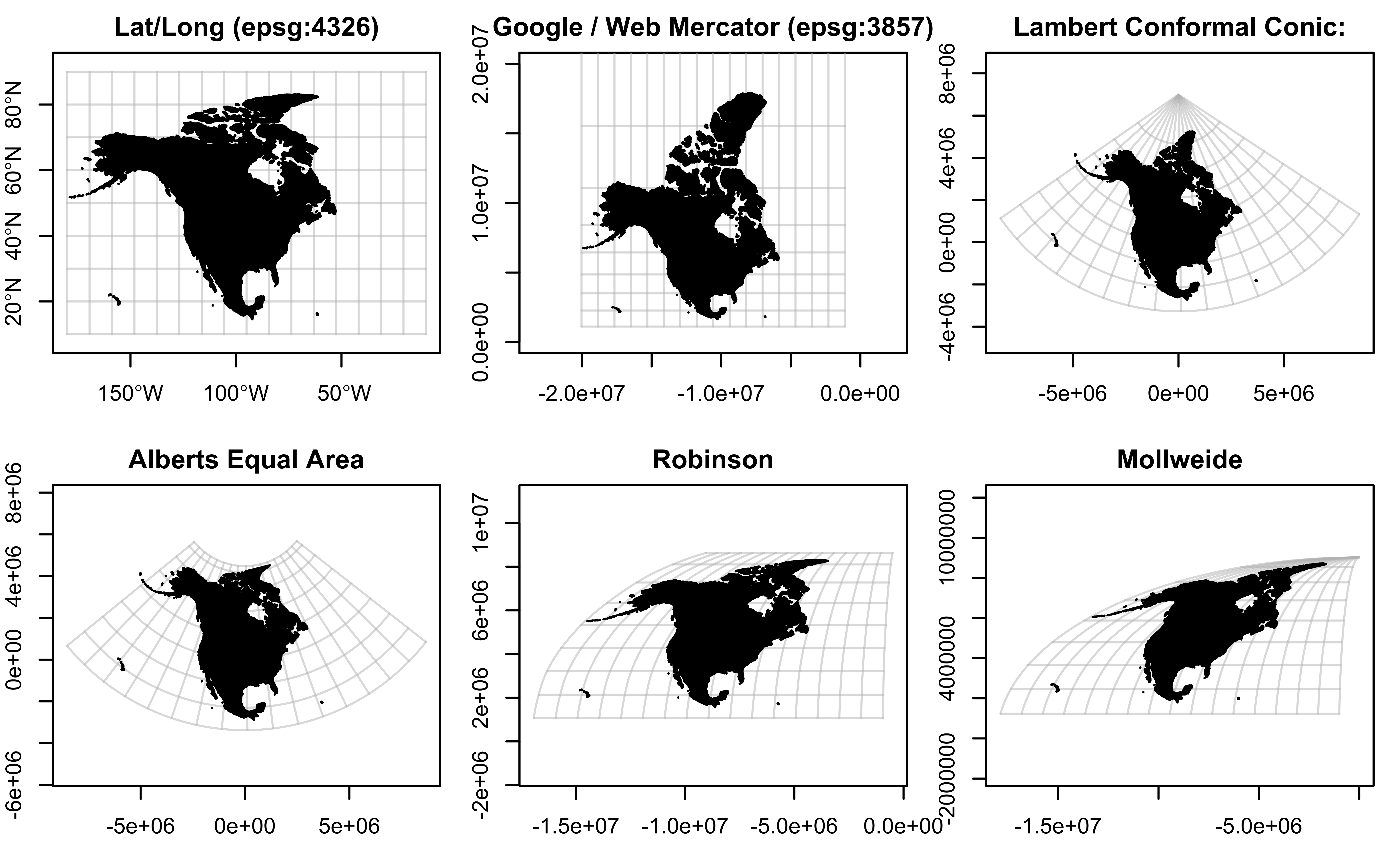
Plotting with Base R

Base R plots

• Created with plot()
• Automatically applied methods based on class of object being plotted

All variables at once

Where did these variables come from? Which of these plots don’t make sense?

plot(nc)

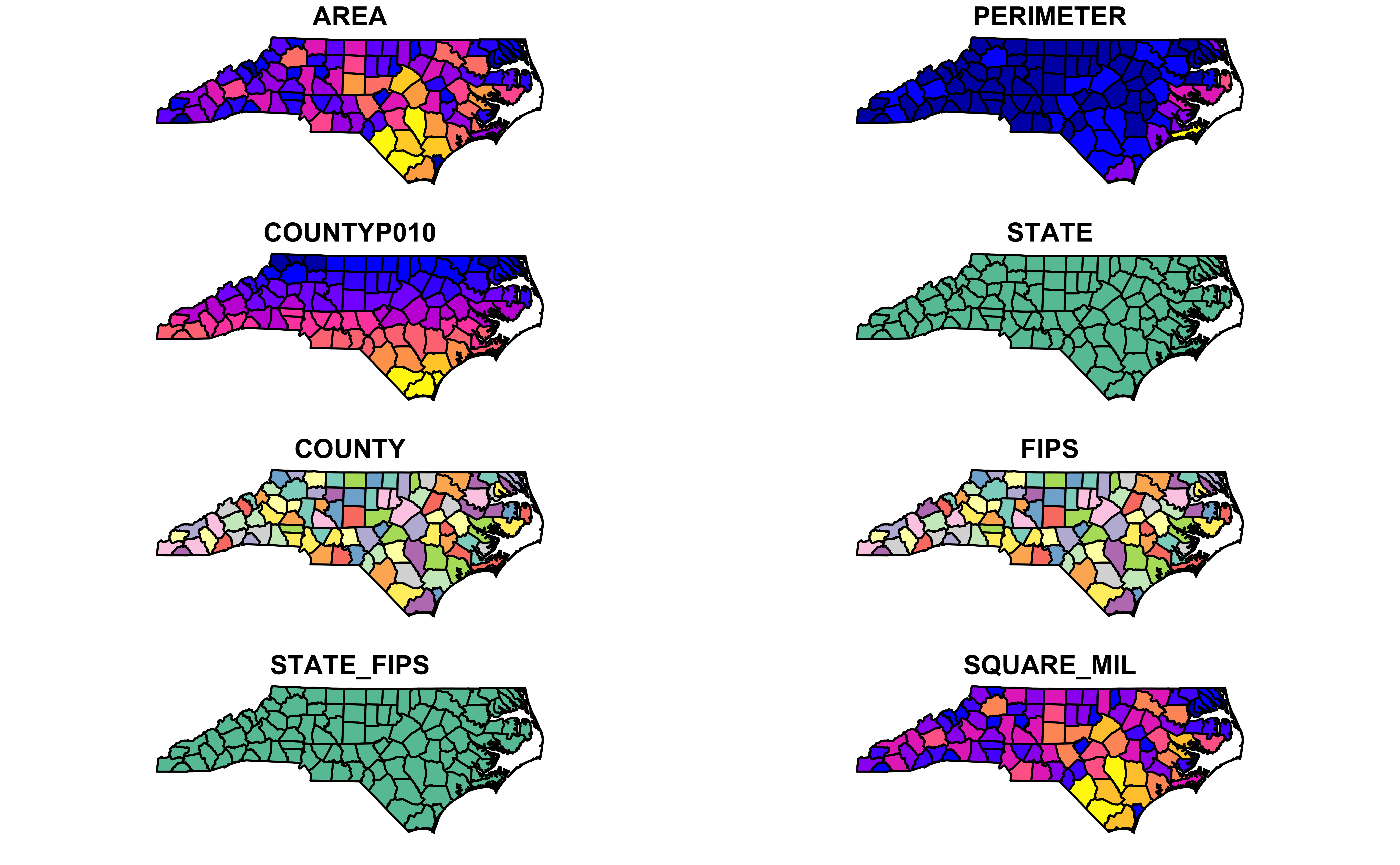
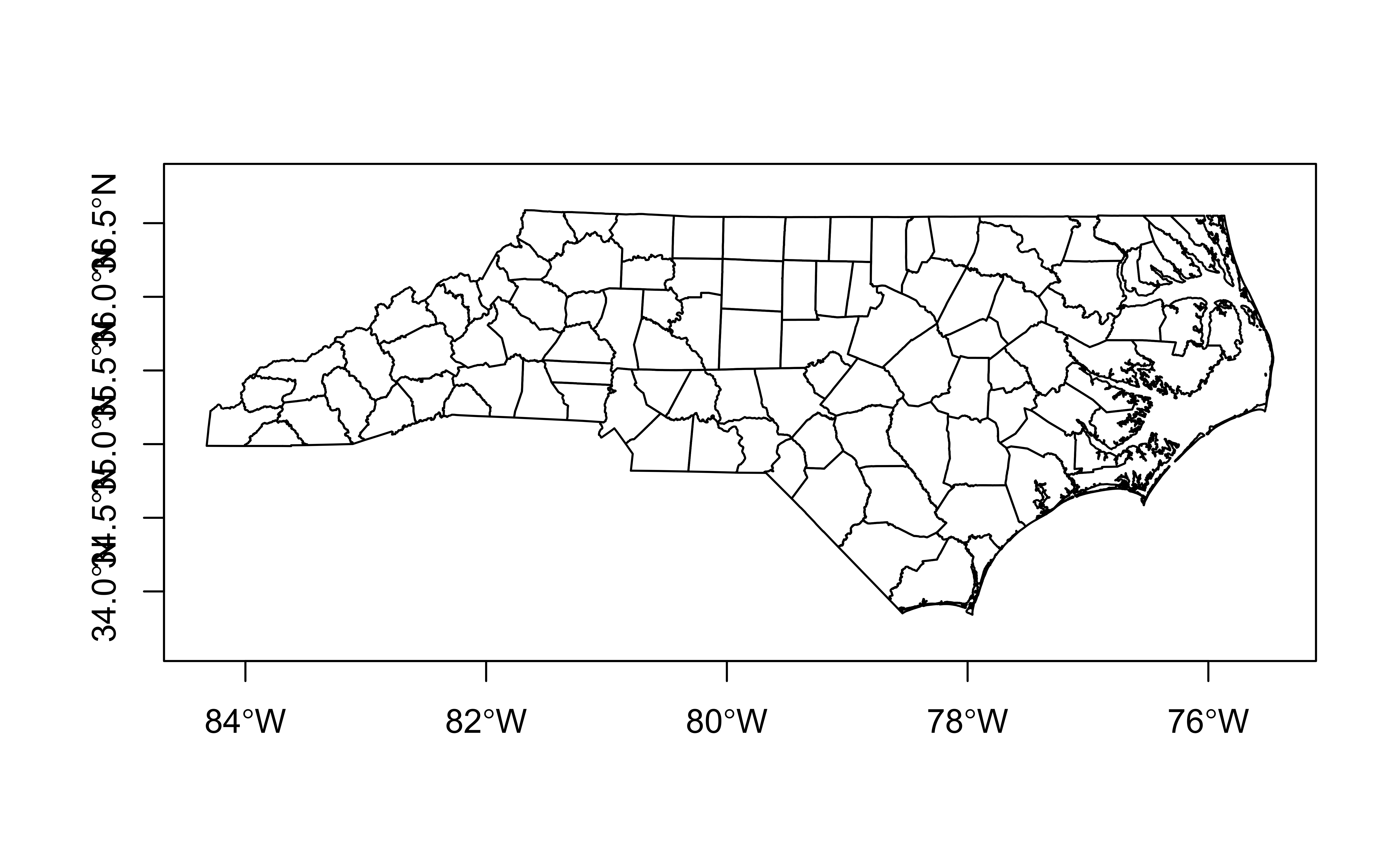
Geometry Plot

plot(st_geometry(nc), axes = TRUE)

Graticules

plot(nc[, "AREA"], axes = TRUE)

Graticules

plot(nc[, "AREA"], graticule = st_crs(nc), axes = TRUE)

Graticules (EPSG:3631)

plot(st_transform(nc[, "AREA"], 3631), axes = TRUE)

Graticules (EPSG:3631)

plot(st_transform(nc[, "AREA"], 3631), graticule = st_crs(nc), axes = TRUE)

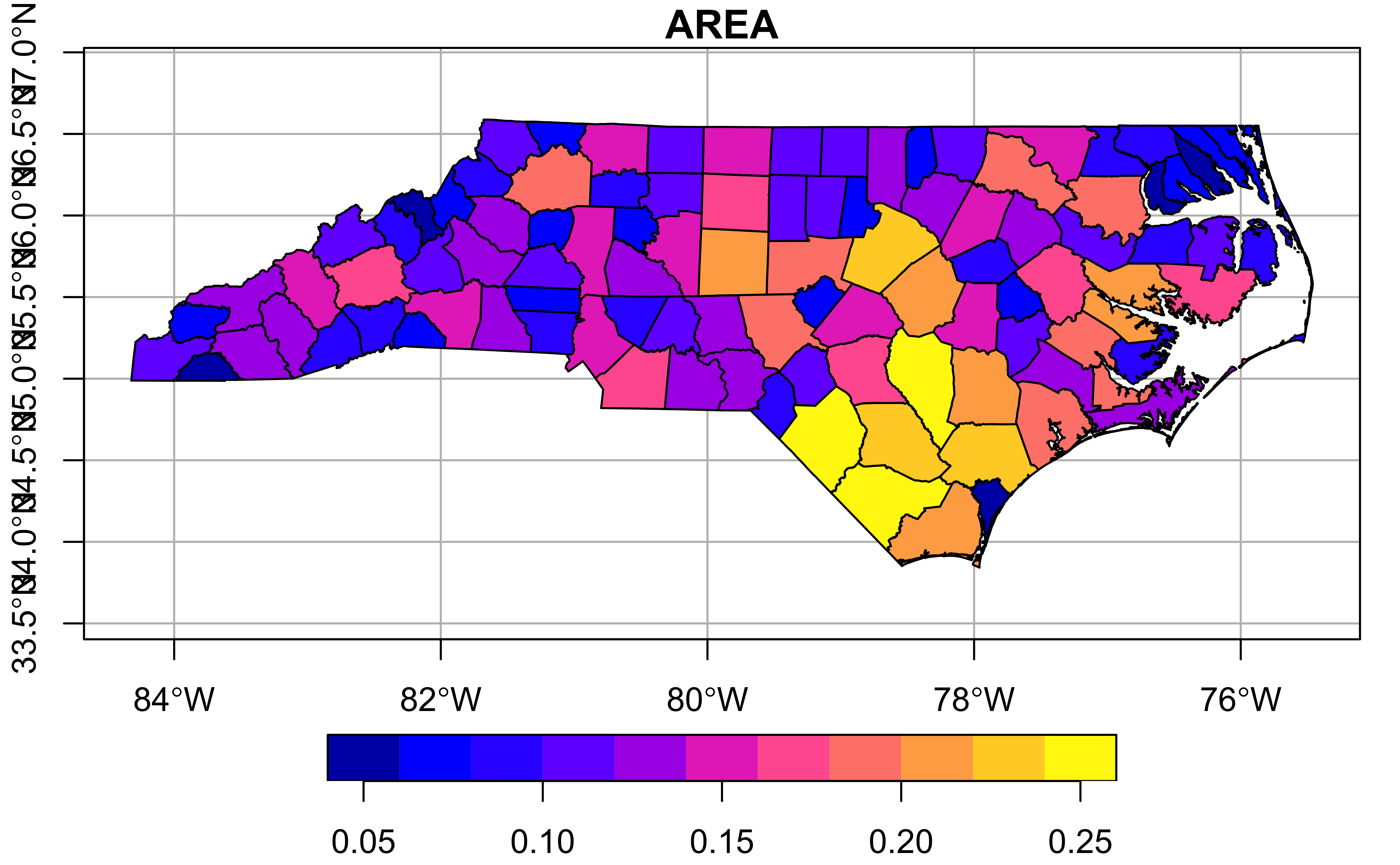
Plotting with ggplot2

geom_sf()

No automatic plotting:

ggplot(nc) +
  geom_sf()

aes()thetic mappings

More expressive: to plot variables, use aesthetic mappings as usual:

ggplot(nc) +
  geom_sf(aes(fill = AREA))

Many variables at once

Using patchwork:

p_area <- ggplot(nc) +
  geom_sf(aes(fill = AREA))
p_perimeter <- ggplot(nc) +
  geom_sf(aes(fill = SQUARE_MIL)) +
  theme(axis.text.y = element_blank())
p_area + p_perimeter

ggplot2 + projections

ggplot(st_transform(nc, 3631)) +
  geom_sf(aes(fill = AREA))

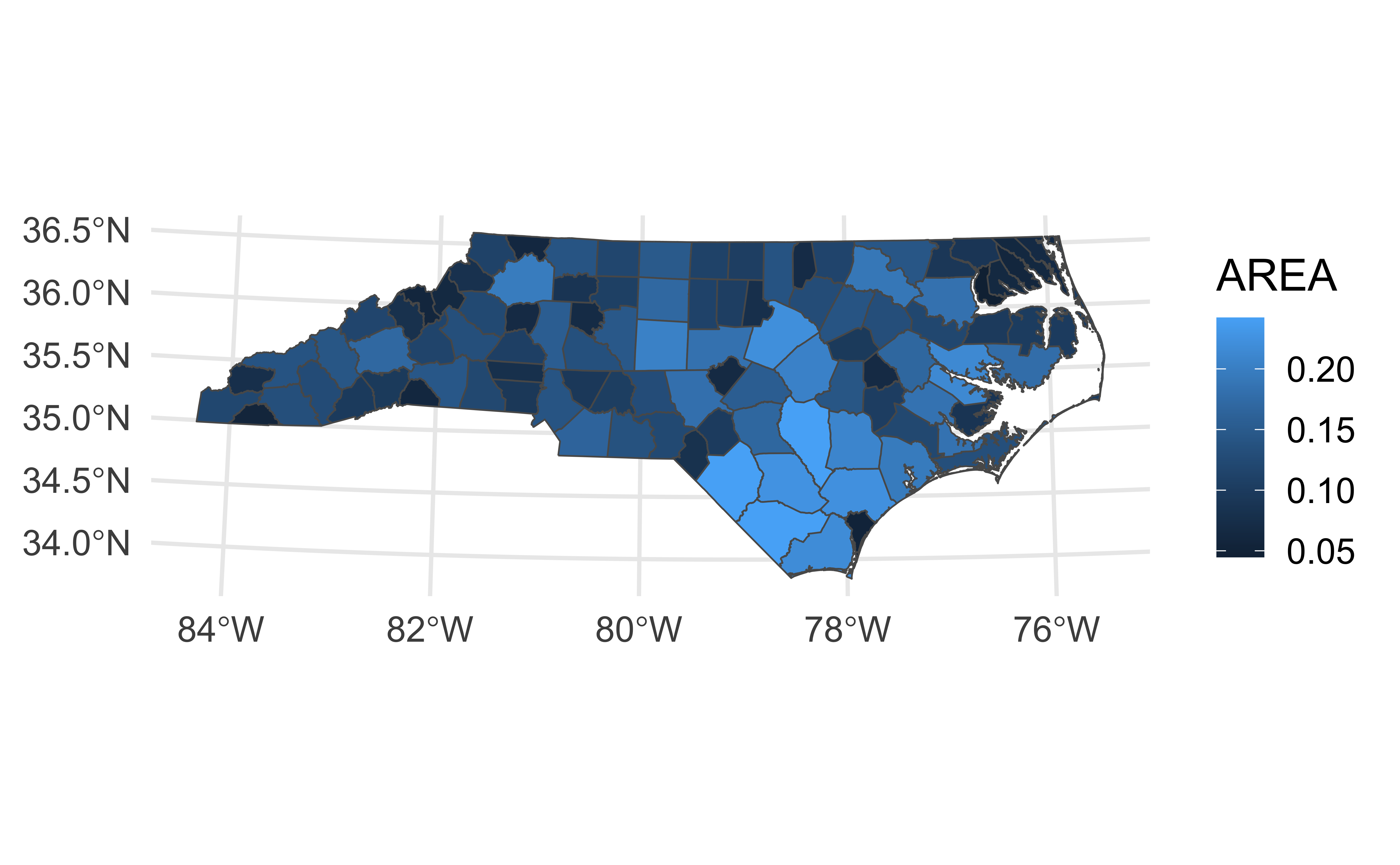
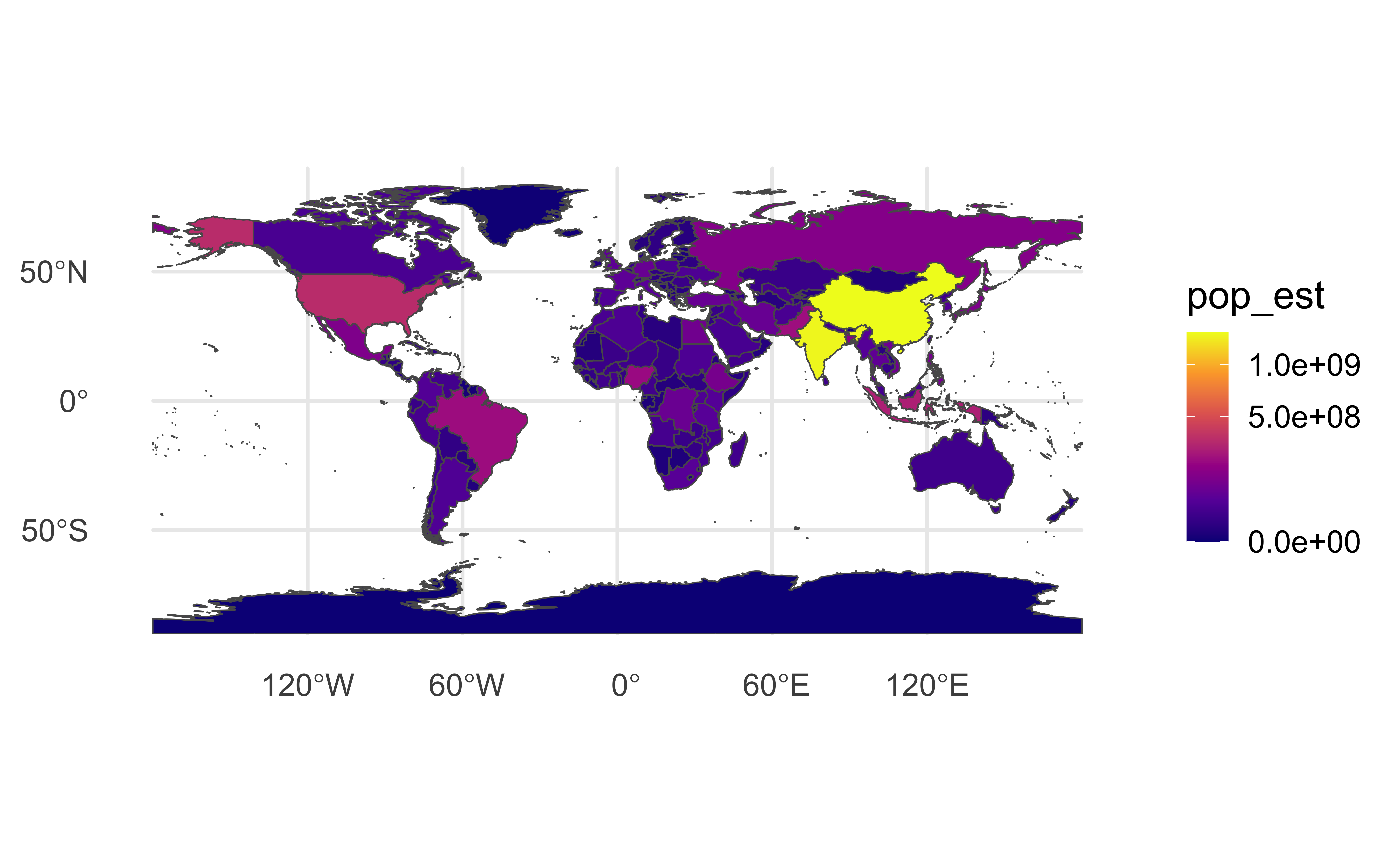
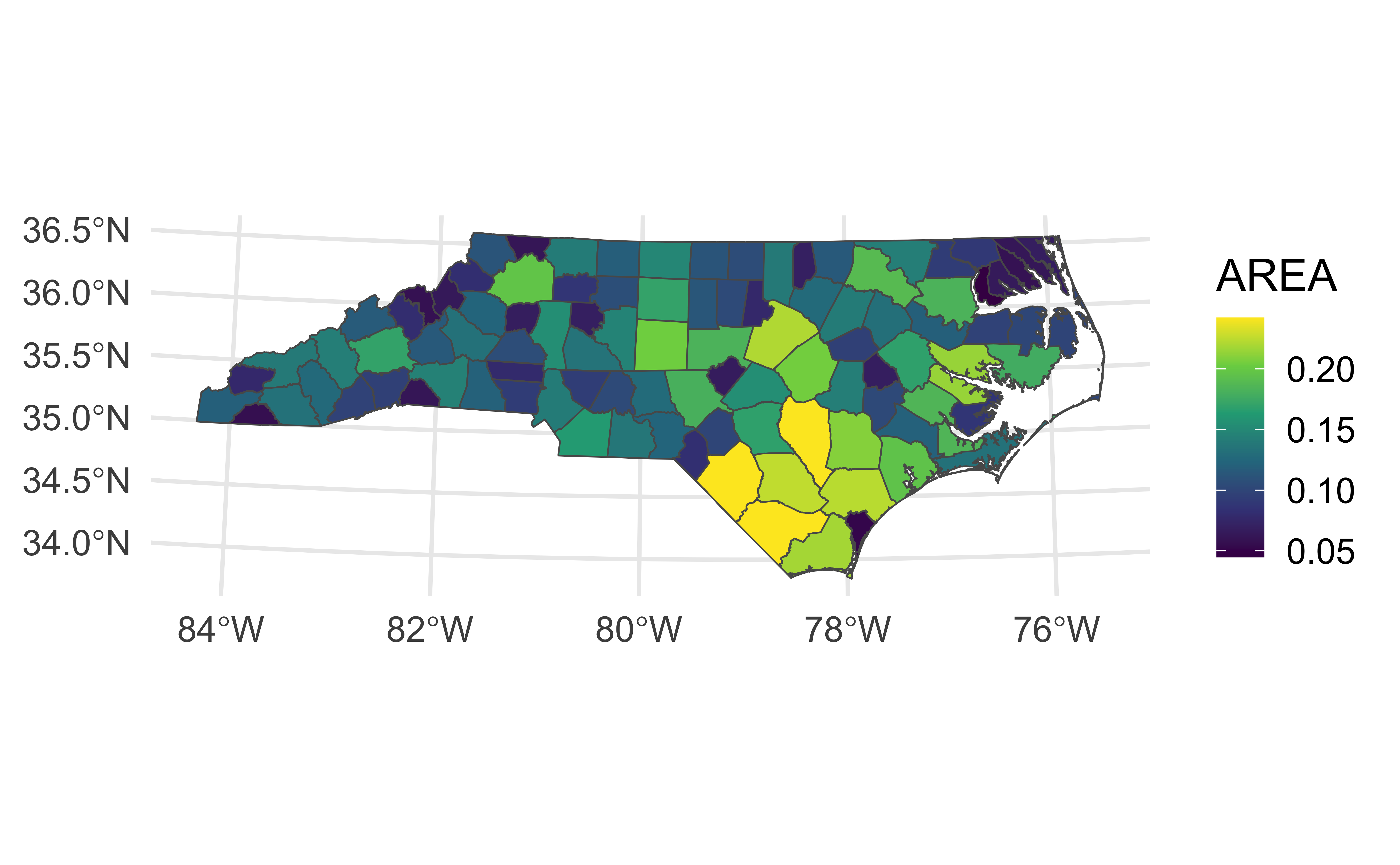
ggplot2 + viridis

ggplot(st_transform(nc, 3631)) +
  geom_sf(aes(fill = AREA)) +
  scale_fill_viridis_c()

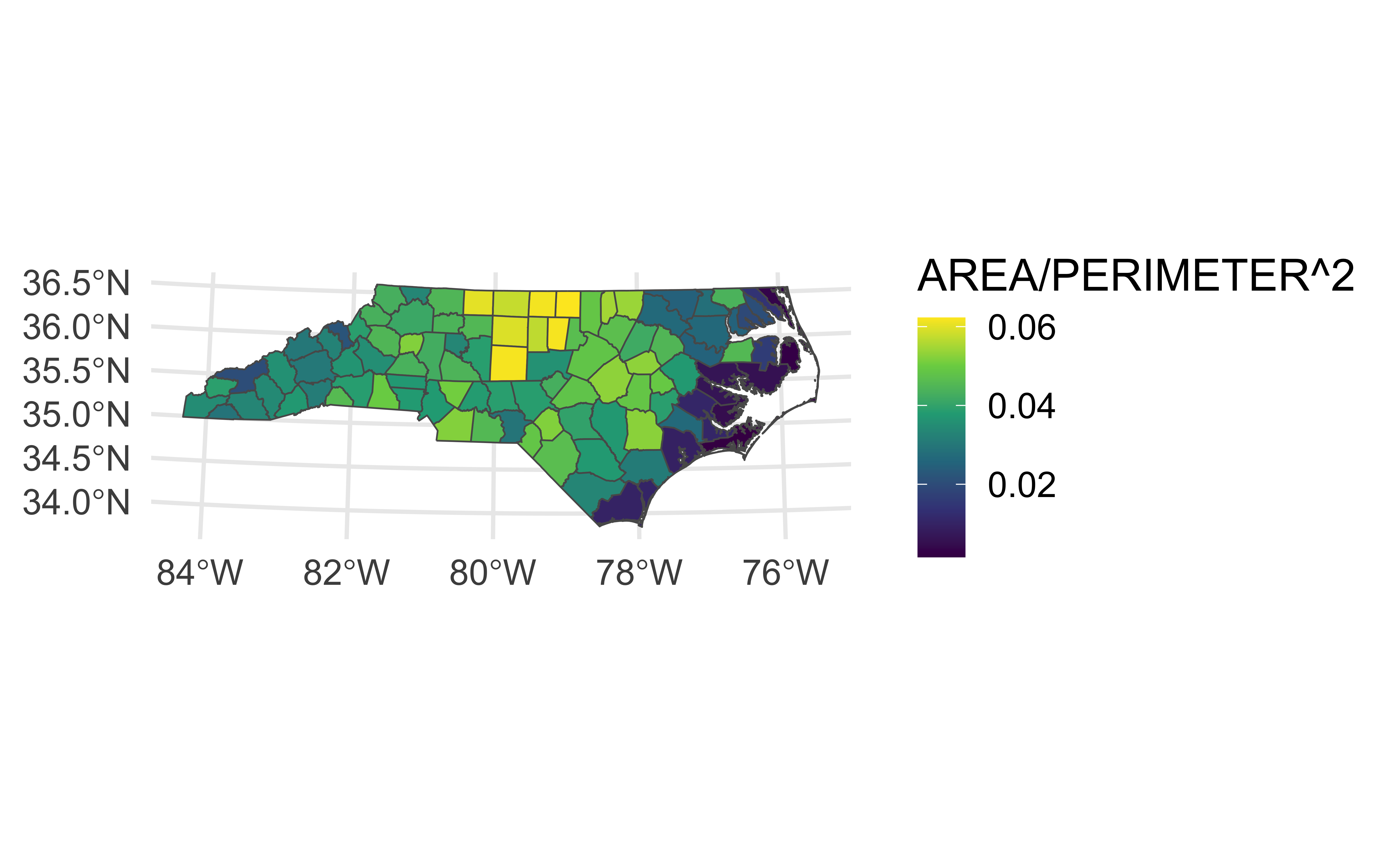
ggplot2 + calculations

ggplot(st_transform(nc, 3631)) +
  geom_sf(aes(fill = AREA / PERIMETER^2)) +
  scale_fill_viridis_c()

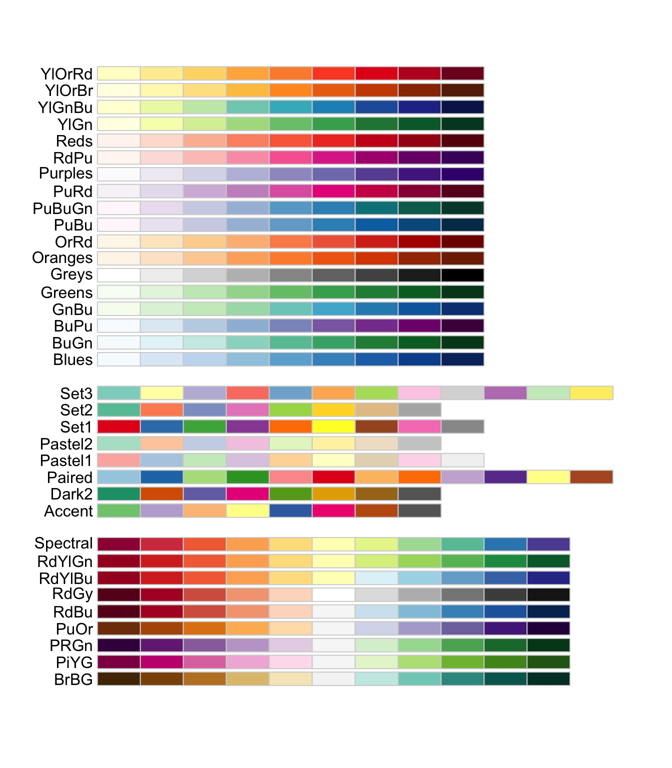
Other color palettes (discrete)

ColorBrewer 2.0 - color advice for maps

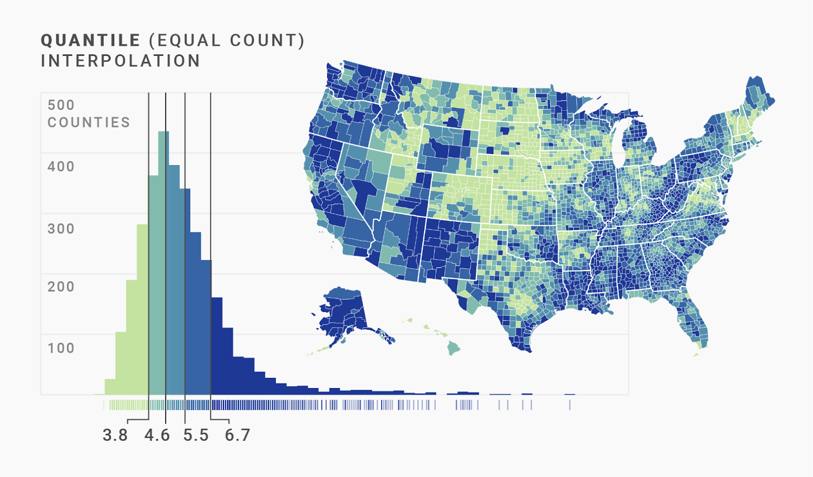
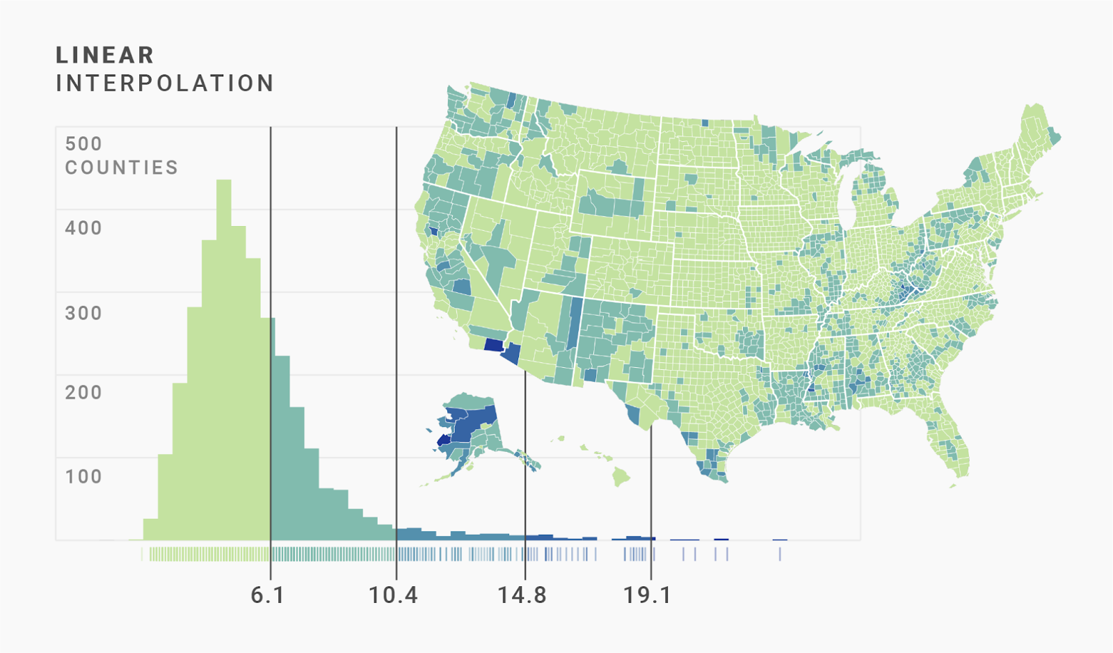
Picking palette breaks

From How to choose an interpolation for your color scale

Picking palette breaks

From How to choose an interpolation for your color scale

Layering maps

Data

ggplot(data = nc) +
  geom_sf() +
  labs(title = "NC Counties")
ggplot(data = air) +
  geom_sf(color = "blue") +
  labs(title = "US Airports")
ggplot(data = hwy) +
  geom_sf(color = "orange") +
  labs(title = "US Highways")

Layering

ae-12 - Part 1: Recreate the following visualization.

Which counties have airports?

nc_airports <- st_intersects(nc, air)
str(nc_airports)

List of 100
 $ : int(0) 
 $ : int(0) 
 $ : int(0) 
 $ : int(0) 
 $ : int(0) 
 $ : int(0) 
 $ : int(0) 
 $ : int(0) 
 $ : int(0) 
 $ : int(0) 
 $ : int(0) 
 $ : int(0) 
 $ : int(0) 
 $ : int(0) 
 $ : int(0) 
 $ : int(0) 
 $ : int(0) 
 $ : int(0) 
 $ : int(0) 
 $ : int(0) 
 $ : int(0) 
 $ : int(0) 
 $ : int(0) 
 $ : int(0) 
 $ : int 268
 $ : int 717
 $ : int(0) 
 $ : int(0) 
 $ : int(0) 
 $ : int(0) 
 $ : int 904
 $ : int(0) 
 $ : int(0) 
 $ : int(0) 
 $ : int(0) 
 $ : int(0) 
 $ : int 764
 $ : int(0) 
 $ : int(0) 
 $ : int(0) 
 $ : int(0) 
 $ : int(0) 
 $ : int(0) 
 $ : int(0) 
 $ : int(0) 
 $ : int(0) 
 $ : int(0) 
 $ : int(0) 
 $ : int(0) 
 $ : int(0) 
 $ : int(0) 
 $ : int 543
 $ : int 892
 $ : int 647
 $ : int(0) 
 $ : int(0) 
 $ : int(0) 
 $ : int(0) 
 $ : int(0) 
 $ : int(0) 
 $ : int(0) 
 $ : int(0) 
 $ : int 176
 $ : int(0) 
 $ : int(0) 
 $ : int(0) 
 $ : int(0) 
 $ : int 789
 $ : int 902
 $ : int(0) 
 $ : int 377
 $ : int(0) 
 $ : int(0) 
 $ : int(0) 
 $ : int 407
 $ : int(0) 
 $ : int(0) 
 $ : int [1:2] 516 593
 $ : int(0) 
 $ : int(0) 
 $ : int(0) 
 $ : int(0) 
 $ : int(0) 
 $ : int [1:2] 491 626
 $ : int(0) 
 $ : int(0) 
 $ : int(0) 
 $ : int(0) 
 $ : int(0) 
 $ : int(0) 
 $ : int(0) 
 $ : int(0) 
 $ : int(0) 
 $ : int 597
 $ : int(0) 
 $ : int(0) 
 $ : int(0) 
 $ : int(0) 
 $ : int 674
  [list output truncated]
 - attr(*, "predicate")= chr "intersects"
 - attr(*, "region.id")= chr [1:100] "1" "2" "3" "4" ...
 - attr(*, "remove_self")= logi FALSE
 - attr(*, "retain_unique")= logi FALSE
 - attr(*, "ncol")= int 940
 - attr(*, "class")= chr [1:2] "sgbp" "list"

Which counties have airports?

has_airport <- map_lgl(nc_airports, ~ length(.) > 0)
nc |>
  slice(which(has_airport)) |>
  pull(COUNTY)

 [1] "Forsyth County"     "Guilford County"    "Dare County"       
 [4] "Wake County"        "Pitt County"        "Catawba County"    
 [7] "Buncombe County"    "Wayne County"       "Mecklenburg County"
[10] "Moore County"       "Cabarrus County"    "Lenoir County"     
[13] "Craven County"      "Cumberland County"  "Onslow County"     
[16] "New Hanover County"

Which counties have airports?

ae-12 - Part 2: On the map of NC you made previously, highlight the counties that have airports.

Using stars

Spatiotemporal arrays with stars

The stars package provides infrastructure for data cubes, array data with labeled dimensions, with emphasis on arrays where some of the dimensions relate to time and/or space.

Three-dimensional cube:

Multi-dimensional hypercube:

Source: https://r-spatial.github.io/stars/

Easter Island

Easter Island (Rapa Nui / Isla de Pascua), a Chilean territory, is a remote volcanic island in Polynesia.

Source: https://en.wikipedia.org/wiki/Easter_Island

File types

• tif files are geospatial raster data, e.g., elevation maps

• gpkg are geopackage files, modern version of shapefiles

Reading tif files

elev <- read_stars("data/easter_island/ei_elev.tif")
elev

stars object with 2 dimensions and 1 attribute
attribute(s):
             Min.  1st Qu.   Median     Mean  3rd Qu.     Max.   NA's
ei_elev.tif     0 56.98041 114.3601 143.5146 204.9752 506.8161 619721
dimension(s):
  from   to  offset delta                refsys point x/y
x    1 1060  651409    25 WGS 84 / UTM zone 12S FALSE [x]
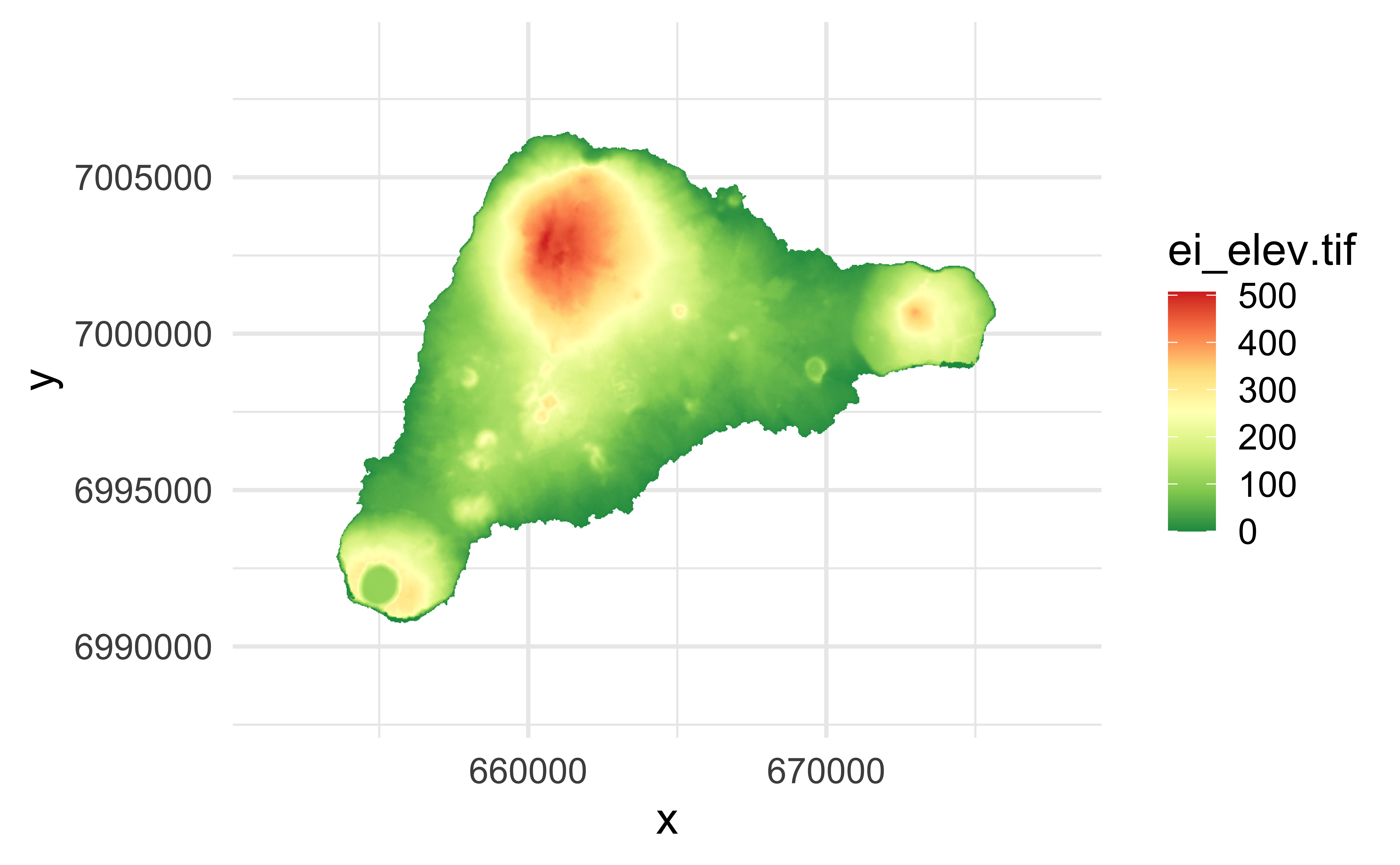
y    1  832 7008921   -25 WGS 84 / UTM zone 12S FALSE [y]

Plotting tif files

ggplot() +
  geom_stars(data = elev)

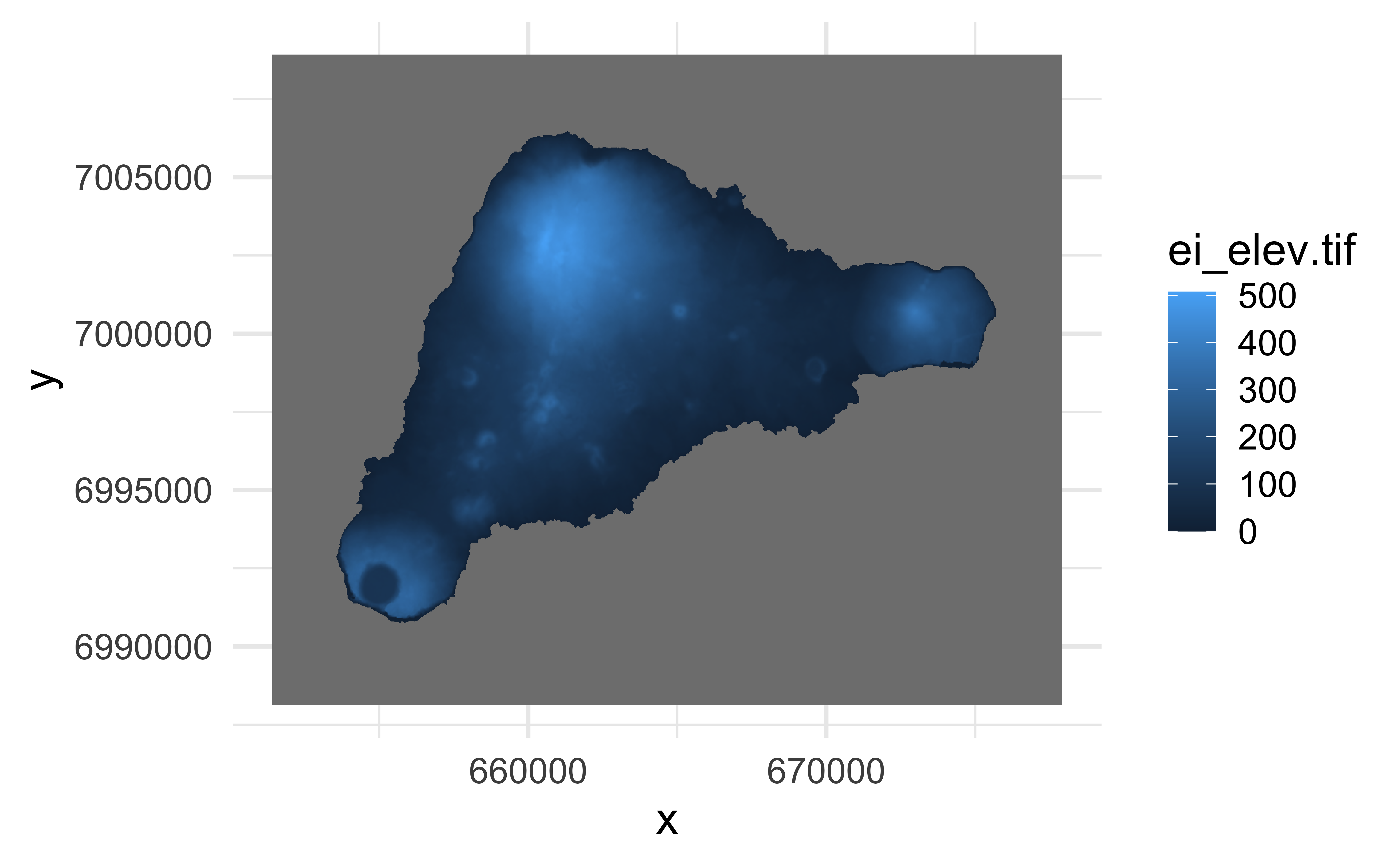
Plays nicely with ggplot2

ggplot() +
  geom_stars(data = elev) +
  scale_fill_distiller(palette = "RdYlGn", na.value = "transparent")

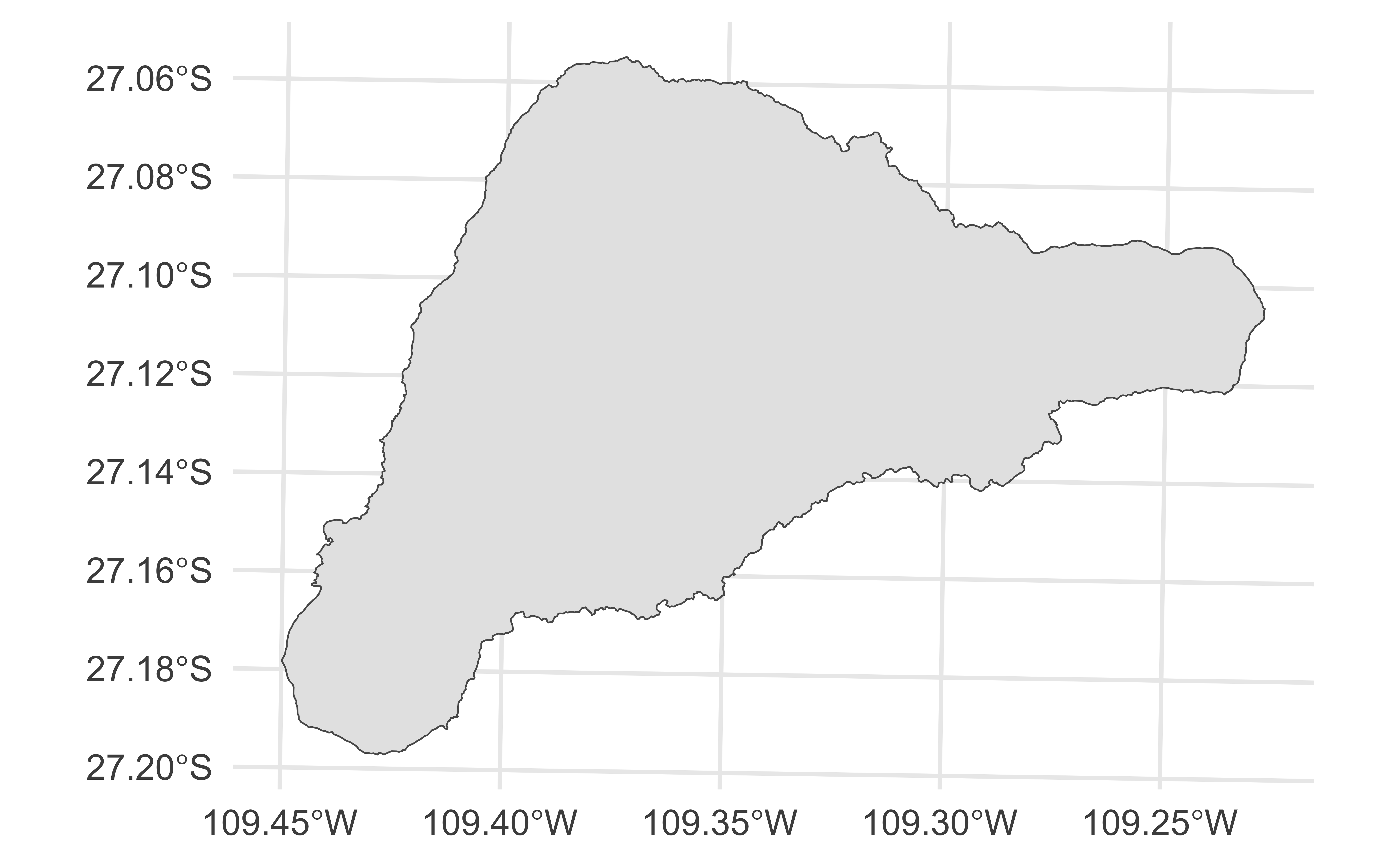
Reading gpkg files

border <- read_sf("data/easter_island/ei_border.gpkg")
border

Simple feature collection with 1 feature and 1 field
Geometry type: POLYGON
Dimension:     XY
Bounding box:  xmin: 653566.4 ymin: 6990751 xmax: 675697.4 ymax: 7006462
Projected CRS: WGS 84 / UTM zone 12S
# A tibble: 1 × 2
  name                                                                      geom
  <chr>                                                            <POLYGON [m]>
1 Rapa Nui / Isla de Pascua ((668715.4 7002628, 668776.6 7002640, 668796 700268…

Plotting gpkg files

ggplot() +
  geom_sf(data = border)

A brief aside…

Put a flag on it!

Just for fun…

ei_plot <- ggplot() +
  geom_sf(data = border, fill = "white")

ei_flag_image <- image_read("images/Flag_of_Rapa_Nui_Chile.png")
ei_flag_raster <- as.raster(ei_flag_image)

ei_plot +
  annotation_raster(
    ei_flag_raster,
    xmin = 657000,
    xmax = 670000,
    ymin = 6996000,
    ymax = 7004000
  )

Source: https://en.wikipedia.org/wiki/Easter_Island

Put a flag on it!

Finding the “bounding box”

• ggplot_build() takes the plot object, and performs all steps necessary to produce an object that can be rendered
• Outputs:
  1. a list of data frames (one for each layer)
  2. a panel object, which contains all information about axis limits, breaks etc.

ei_plot_build <- ggplot_build(ei_plot)

ggplot_build()

ei_plot_build

<ggplot2::ggplot_built>
 @ data  :List of 1
 .. $ :'data.frame':    1 obs. of  13 variables:
 ..  ..$ geometry :sfc_POLYGON of length 1; first list element: List of 1
 ..  .. ..$ : num [1:1072, 1:2] 668715 668777 668796 668860 668916 ...
 ..  .. ..- attr(*, "class")= chr [1:3] "XY" "POLYGON" "sfg"
 ..  ..$ PANEL    : Factor w/ 1 level "1": 1
 ..  ..$ group    : int -1
 ..  .. ..- attr(*, "n")= int 1
 ..  ..$ xmin     : num 653566
 ..  ..$ xmax     : num 675697
 ..  ..$ ymin     : num 6990751
 ..  ..$ ymax     : num 7006462
 ..  ..$ linetype : int 1
 ..  ..$ alpha    : logi NA
 ..  ..$ stroke   : num 0.5
 ..  ..$ fill     : chr "white"
 ..  ..$ colour   : chr "#595959FF"
 ..  ..$ linewidth: num 0.291
 @ layout:Classes 'Layout', 'ggproto', 'gg' <ggproto object: Class Layout, gg>
    coord: <ggproto object: Class CoordSf, CoordCartesian, Coord, gg>
        aspect: function
        backtransform_range: function
        clip: on
        crs: NULL
        datum: crs
        default: TRUE
        default_crs: NULL
        determine_crs: function
        distance: function
        draw_panel: function
        expand: TRUE
        fixup_graticule_labels: function
        get_default_crs: function
        is_free: function
        is_linear: function
        label_axes: list
        label_graticule: 
        labels: function
        limits: list
        lims_method: cross
        modify_scales: function
        ndiscr: 100
        params: list
        range: function
        record_bbox: function
        render_axis_h: function
        render_axis_v: function
        render_bg: function
        render_fg: function
        reverse: none
        setup_data: function
        setup_layout: function
        setup_panel_guides: function
        setup_panel_params: function
        setup_params: function
        train_panel_guides: function
        transform: function
        super:  <ggproto object: Class CoordSf, CoordCartesian, Coord, gg>
    coord_params: list
    facet: <ggproto object: Class FacetNull, Facet, gg>
        attach_axes: function
        attach_strips: function
        compute_layout: function
        draw_back: function
        draw_front: function
        draw_labels: function
        draw_panel_content: function
        draw_panels: function
        finish_data: function
        format_strip_labels: function
        init_gtable: function
        init_scales: function
        map_data: function
        params: list
        set_panel_size: function
        setup_data: function
        setup_panel_params: function
        setup_params: function
        shrink: TRUE
        train_scales: function
        vars: function
        super:  <ggproto object: Class FacetNull, Facet, gg>
    facet_params: list
    finish_data: function
    get_scales: function
    layout: data.frame
    map_position: function
    panel_params: list
    panel_scales_x: list
    panel_scales_y: list
    render: function
    render_labels: function
    reset_scales: function
    resolve_label: function
    setup: function
    setup_panel_guides: function
    setup_panel_params: function
    train_position: function
    super:  <ggproto object: Class Layout, gg> 
 @ plot  : <ggplot2::ggplot>
 .. @ data       : list()
 .. .. - attr(*, "class")= chr "waiver"
 .. @ layers     :List of 1
 .. .. $ geom_sf:Classes 'LayerInstance', 'LayerSf', 'Layer', 'ggproto', 'gg' <ggproto object: Class LayerInstance, LayerSf, Layer, gg>
    aes_params: list
    compute_aesthetics: function
    compute_geom_1: function
    compute_geom_2: function
    compute_position: function
    compute_statistic: function
    computed_geom_params: list
    computed_mapping: ggplot2::mapping, uneval, gg, S7_object
    computed_stat_params: list
    constructor: call
    data: sf, tbl_df, tbl, data.frame
    draw_geom: function
    finish_statistics: function
    geom: <ggproto object: Class GeomSf, Geom, gg>
        aesthetics: function
        default_aes: ggplot2::mapping, uneval, gg, S7_object
        draw_group: function
        draw_key: function
        draw_layer: function
        draw_panel: function
        extra_params: na.rm
        handle_na: function
        non_missing_aes: 
        optional_aes: 
        parameters: function
        rename_size: FALSE
        required_aes: geometry
        setup_data: function
        setup_params: function
        use_defaults: function
        super:  <ggproto object: Class Geom, gg>
    geom_params: list
    inherit.aes: TRUE
    layer_data: function
    layout: NULL
    legend_key_type: NULL
    map_statistic: function
    mapping: ggplot2::mapping, uneval, gg, S7_object
    name: NULL
    position: <ggproto object: Class PositionIdentity, Position, gg>
        aesthetics: function
        compute_layer: function
        compute_panel: function
        default_aes: ggplot2::mapping, uneval, gg, S7_object
        required_aes: 
        setup_data: function
        setup_params: function
        use_defaults: function
        super:  <ggproto object: Class Position, gg>
    print: function
    setup_layer: function
    show.legend: NA
    stat: <ggproto object: Class StatSf, Stat, gg>
        aesthetics: function
        compute_group: function
        compute_layer: function
        compute_panel: function
        default_aes: ggplot2::mapping, uneval, gg, S7_object
        dropped_aes: 
        extra_params: na.rm
        finish_layer: function
        non_missing_aes: 
        optional_aes: 
        parameters: function
        required_aes: geometry
        retransform: TRUE
        setup_data: function
        setup_params: function
        super:  <ggproto object: Class Stat, gg>
    stat_params: list
    super:  <ggproto object: Class LayerSf, Layer, gg> 
 .. @ scales     :Classes 'ScalesList', 'ggproto', 'gg' <ggproto object: Class ScalesList, gg>
    add: function
    add_defaults: function
    add_missing: function
    backtransform_df: function
    clone: function
    find: function
    get_scales: function
    has_scale: function
    input: function
    map_df: function
    n: function
    non_position_scales: function
    scales: list
    set_palettes: function
    train_df: function
    transform_df: function
    super:  <ggproto object: Class ScalesList, gg> 
 .. @ guides     :Classes 'Guides', 'ggproto', 'gg' <ggproto object: Class Guides, gg>
    add: function
    assemble: function
    build: function
    draw: function
    get_custom: function
    get_guide: function
    get_params: function
    get_position: function
    guides: NULL
    merge: function
    missing: <ggproto object: Class GuideNone, Guide, gg>
        add_title: function
        arrange_layout: function
        assemble_drawing: function
        available_aes: any
        build_decor: function
        build_labels: function
        build_ticks: function
        build_title: function
        draw: function
        draw_early_exit: function
        elements: list
        extract_decor: function
        extract_key: function
        extract_params: function
        get_layer_key: function
        hashables: list
        measure_grobs: function
        merge: function
        override_elements: function
        params: list
        process_layers: function
        setup_elements: function
        setup_params: function
        train: function
        transform: function
        super:  <ggproto object: Class GuideNone, Guide, gg>
    package_box: function
    print: function
    process_layers: function
    setup: function
    subset_guides: function
    train: function
    update_params: function
    super:  <ggproto object: Class Guides, gg> 
 .. @ mapping    : <ggplot2::mapping>  Named list()
 .. @ theme      : <theme> List of 144
 .. .. $ line                            : <ggplot2::element_line>
 .. ..  ..@ colour       : chr "black"
 .. ..  ..@ linewidth    : num 0.727
 .. ..  ..@ linetype     : num 1
 .. ..  ..@ lineend      : chr "butt"
 .. ..  ..@ linejoin     : chr "round"
 .. ..  ..@ arrow        : logi FALSE
 .. ..  ..@ arrow.fill   : chr "black"
 .. ..  ..@ inherit.blank: logi TRUE
 .. .. $ rect                            : <ggplot2::element_rect>
 .. ..  ..@ fill         : chr "white"
 .. ..  ..@ colour       : chr "black"
 .. ..  ..@ linewidth    : num 0.727
 .. ..  ..@ linetype     : num 1
 .. ..  ..@ linejoin     : chr "round"
 .. ..  ..@ inherit.blank: logi TRUE
 .. .. $ text                            : <ggplot2::element_text>
 .. ..  ..@ family       : chr ""
 .. ..  ..@ face         : chr "plain"
 .. ..  ..@ italic       : chr NA
 .. ..  ..@ fontweight   : num NA
 .. ..  ..@ fontwidth    : num NA
 .. ..  ..@ colour       : chr "black"
 .. ..  ..@ size         : num 16
 .. ..  ..@ hjust        : num 0.5
 .. ..  ..@ vjust        : num 0.5
 .. ..  ..@ angle        : num 0
 .. ..  ..@ lineheight   : num 0.9
 .. ..  ..@ margin       : <ggplot2::margin> num [1:4] 0 0 0 0
 .. ..  ..@ debug        : logi FALSE
 .. ..  ..@ inherit.blank: logi TRUE
 .. .. $ title                           : <ggplot2::element_text>
 .. ..  ..@ family       : NULL
 .. ..  ..@ face         : NULL
 .. ..  ..@ italic       : chr NA
 .. ..  ..@ fontweight   : num NA
 .. ..  ..@ fontwidth    : num NA
 .. ..  ..@ colour       : NULL
 .. ..  ..@ size         : NULL
 .. ..  ..@ hjust        : NULL
 .. ..  ..@ vjust        : NULL
 .. ..  ..@ angle        : NULL
 .. ..  ..@ lineheight   : NULL
 .. ..  ..@ margin       : NULL
 .. ..  ..@ debug        : NULL
 .. ..  ..@ inherit.blank: logi TRUE
 .. .. $ point                           : <ggplot2::element_point>
 .. ..  ..@ colour       : chr "black"
 .. ..  ..@ shape        : num 19
 .. ..  ..@ size         : num 2.18
 .. ..  ..@ fill         : chr "white"
 .. ..  ..@ stroke       : num 0.727
 .. ..  ..@ inherit.blank: logi TRUE
 .. .. $ polygon                         : <ggplot2::element_polygon>
 .. ..  ..@ fill         : chr "white"
 .. ..  ..@ colour       : chr "black"
 .. ..  ..@ linewidth    : num 0.727
 .. ..  ..@ linetype     : num 1
 .. ..  ..@ linejoin     : chr "round"
 .. ..  ..@ inherit.blank: logi TRUE
 .. .. $ geom                            : <ggplot2::element_geom>
 .. ..  ..@ ink        : chr "black"
 .. ..  ..@ paper      : chr "white"
 .. ..  ..@ accent     : chr "#3366FF"
 .. ..  ..@ linewidth  : num 0.727
 .. ..  ..@ borderwidth: num 0.727
 .. ..  ..@ linetype   : int 1
 .. ..  ..@ bordertype : int 1
 .. ..  ..@ family     : chr ""
 .. ..  ..@ fontsize   : num 5.62
 .. ..  ..@ pointsize  : num 2.18
 .. ..  ..@ pointshape : num 19
 .. ..  ..@ colour     : NULL
 .. ..  ..@ fill       : NULL
 .. .. $ spacing                         : 'simpleUnit' num 8points
 .. ..  ..- attr(*, "unit")= int 8
 .. .. $ margins                         : <ggplot2::margin> num [1:4] 8 8 8 8
 .. .. $ aspect.ratio                    : NULL
 .. .. $ axis.title                      : NULL
 .. .. $ axis.title.x                    : <ggplot2::element_text>
 .. ..  ..@ family       : NULL
 .. ..  ..@ face         : NULL
 .. ..  ..@ italic       : chr NA
 .. ..  ..@ fontweight   : num NA
 .. ..  ..@ fontwidth    : num NA
 .. ..  ..@ colour       : NULL
 .. ..  ..@ size         : NULL
 .. ..  ..@ hjust        : NULL
 .. ..  ..@ vjust        : num 1
 .. ..  ..@ angle        : NULL
 .. ..  ..@ lineheight   : NULL
 .. ..  ..@ margin       : <ggplot2::margin> num [1:4] 4 0 0 0
 .. ..  ..@ debug        : NULL
 .. ..  ..@ inherit.blank: logi TRUE
 .. .. $ axis.title.x.top                : <ggplot2::element_text>
 .. ..  ..@ family       : NULL
 .. ..  ..@ face         : NULL
 .. ..  ..@ italic       : chr NA
 .. ..  ..@ fontweight   : num NA
 .. ..  ..@ fontwidth    : num NA
 .. ..  ..@ colour       : NULL
 .. ..  ..@ size         : NULL
 .. ..  ..@ hjust        : NULL
 .. ..  ..@ vjust        : num 0
 .. ..  ..@ angle        : NULL
 .. ..  ..@ lineheight   : NULL
 .. ..  ..@ margin       : <ggplot2::margin> num [1:4] 0 0 4 0
 .. ..  ..@ debug        : NULL
 .. ..  ..@ inherit.blank: logi TRUE
 .. .. $ axis.title.x.bottom             : NULL
 .. .. $ axis.title.y                    : <ggplot2::element_text>
 .. ..  ..@ family       : NULL
 .. ..  ..@ face         : NULL
 .. ..  ..@ italic       : chr NA
 .. ..  ..@ fontweight   : num NA
 .. ..  ..@ fontwidth    : num NA
 .. ..  ..@ colour       : NULL
 .. ..  ..@ size         : NULL
 .. ..  ..@ hjust        : NULL
 .. ..  ..@ vjust        : num 1
 .. ..  ..@ angle        : num 90
 .. ..  ..@ lineheight   : NULL
 .. ..  ..@ margin       : <ggplot2::margin> num [1:4] 0 4 0 0
 .. ..  ..@ debug        : NULL
 .. ..  ..@ inherit.blank: logi TRUE
 .. .. $ axis.title.y.left               : NULL
 .. .. $ axis.title.y.right              : <ggplot2::element_text>
 .. ..  ..@ family       : NULL
 .. ..  ..@ face         : NULL
 .. ..  ..@ italic       : chr NA
 .. ..  ..@ fontweight   : num NA
 .. ..  ..@ fontwidth    : num NA
 .. ..  ..@ colour       : NULL
 .. ..  ..@ size         : NULL
 .. ..  ..@ hjust        : NULL
 .. ..  ..@ vjust        : num 1
 .. ..  ..@ angle        : num -90
 .. ..  ..@ lineheight   : NULL
 .. ..  ..@ margin       : <ggplot2::margin> num [1:4] 0 0 0 4
 .. ..  ..@ debug        : NULL
 .. ..  ..@ inherit.blank: logi TRUE
 .. .. $ axis.text                       : <ggplot2::element_text>
 .. ..  ..@ family       : NULL
 .. ..  ..@ face         : NULL
 .. ..  ..@ italic       : chr NA
 .. ..  ..@ fontweight   : num NA
 .. ..  ..@ fontwidth    : num NA
 .. ..  ..@ colour       : chr "#4D4D4DFF"
 .. ..  ..@ size         : 'rel' num 0.8
 .. ..  ..@ hjust        : NULL
 .. ..  ..@ vjust        : NULL
 .. ..  ..@ angle        : NULL
 .. ..  ..@ lineheight   : NULL
 .. ..  ..@ margin       : NULL
 .. ..  ..@ debug        : NULL
 .. ..  ..@ inherit.blank: logi TRUE
 .. .. $ axis.text.x                     : <ggplot2::element_text>
 .. ..  ..@ family       : NULL
 .. ..  ..@ face         : NULL
 .. ..  ..@ italic       : chr NA
 .. ..  ..@ fontweight   : num NA
 .. ..  ..@ fontwidth    : num NA
 .. ..  ..@ colour       : NULL
 .. ..  ..@ size         : NULL
 .. ..  ..@ hjust        : NULL
 .. ..  ..@ vjust        : num 1
 .. ..  ..@ angle        : NULL
 .. ..  ..@ lineheight   : NULL
 .. ..  ..@ margin       : <ggplot2::margin> num [1:4] 3.2 0 0 0
 .. ..  ..@ debug        : NULL
 .. ..  ..@ inherit.blank: logi TRUE
 .. .. $ axis.text.x.top                 : <ggplot2::element_text>
 .. ..  ..@ family       : NULL
 .. ..  ..@ face         : NULL
 .. ..  ..@ italic       : chr NA
 .. ..  ..@ fontweight   : num NA
 .. ..  ..@ fontwidth    : num NA
 .. ..  ..@ colour       : NULL
 .. ..  ..@ size         : NULL
 .. ..  ..@ hjust        : NULL
 .. ..  ..@ vjust        : NULL
 .. ..  ..@ angle        : NULL
 .. ..  ..@ lineheight   : NULL
 .. ..  ..@ margin       : <ggplot2::margin> num [1:4] 0 0 7.2 0
 .. ..  ..@ debug        : NULL
 .. ..  ..@ inherit.blank: logi TRUE
 .. .. $ axis.text.x.bottom              : <ggplot2::element_text>
 .. ..  ..@ family       : NULL
 .. ..  ..@ face         : NULL
 .. ..  ..@ italic       : chr NA
 .. ..  ..@ fontweight   : num NA
 .. ..  ..@ fontwidth    : num NA
 .. ..  ..@ colour       : NULL
 .. ..  ..@ size         : NULL
 .. ..  ..@ hjust        : NULL
 .. ..  ..@ vjust        : NULL
 .. ..  ..@ angle        : NULL
 .. ..  ..@ lineheight   : NULL
 .. ..  ..@ margin       : <ggplot2::margin> num [1:4] 7.2 0 0 0
 .. ..  ..@ debug        : NULL
 .. ..  ..@ inherit.blank: logi TRUE
 .. .. $ axis.text.y                     : <ggplot2::element_text>
 .. ..  ..@ family       : NULL
 .. ..  ..@ face         : NULL
 .. ..  ..@ italic       : chr NA
 .. ..  ..@ fontweight   : num NA
 .. ..  ..@ fontwidth    : num NA
 .. ..  ..@ colour       : NULL
 .. ..  ..@ size         : NULL
 .. ..  ..@ hjust        : num 1
 .. ..  ..@ vjust        : NULL
 .. ..  ..@ angle        : NULL
 .. ..  ..@ lineheight   : NULL
 .. ..  ..@ margin       : <ggplot2::margin> num [1:4] 0 3.2 0 0
 .. ..  ..@ debug        : NULL
 .. ..  ..@ inherit.blank: logi TRUE
 .. .. $ axis.text.y.left                : <ggplot2::element_text>
 .. ..  ..@ family       : NULL
 .. ..  ..@ face         : NULL
 .. ..  ..@ italic       : chr NA
 .. ..  ..@ fontweight   : num NA
 .. ..  ..@ fontwidth    : num NA
 .. ..  ..@ colour       : NULL
 .. ..  ..@ size         : NULL
 .. ..  ..@ hjust        : NULL
 .. ..  ..@ vjust        : NULL
 .. ..  ..@ angle        : NULL
 .. ..  ..@ lineheight   : NULL
 .. ..  ..@ margin       : <ggplot2::margin> num [1:4] 0 7.2 0 0
 .. ..  ..@ debug        : NULL
 .. ..  ..@ inherit.blank: logi TRUE
 .. .. $ axis.text.y.right               : <ggplot2::element_text>
 .. ..  ..@ family       : NULL
 .. ..  ..@ face         : NULL
 .. ..  ..@ italic       : chr NA
 .. ..  ..@ fontweight   : num NA
 .. ..  ..@ fontwidth    : num NA
 .. ..  ..@ colour       : NULL
 .. ..  ..@ size         : NULL
 .. ..  ..@ hjust        : NULL
 .. ..  ..@ vjust        : NULL
 .. ..  ..@ angle        : NULL
 .. ..  ..@ lineheight   : NULL
 .. ..  ..@ margin       : <ggplot2::margin> num [1:4] 0 0 0 7.2
 .. ..  ..@ debug        : NULL
 .. ..  ..@ inherit.blank: logi TRUE
 .. .. $ axis.text.theta                 : NULL
 .. .. $ axis.text.r                     : <ggplot2::element_text>
 .. ..  ..@ family       : NULL
 .. ..  ..@ face         : NULL
 .. ..  ..@ italic       : chr NA
 .. ..  ..@ fontweight   : num NA
 .. ..  ..@ fontwidth    : num NA
 .. ..  ..@ colour       : NULL
 .. ..  ..@ size         : NULL
 .. ..  ..@ hjust        : num 0.5
 .. ..  ..@ vjust        : NULL
 .. ..  ..@ angle        : NULL
 .. ..  ..@ lineheight   : NULL
 .. ..  ..@ margin       : <ggplot2::margin> num [1:4] 0 3.2 0 3.2
 .. ..  ..@ debug        : NULL
 .. ..  ..@ inherit.blank: logi TRUE
 .. .. $ axis.ticks                      : <ggplot2::element_blank>
 .. .. $ axis.ticks.x                    : NULL
 .. .. $ axis.ticks.x.top                : NULL
 .. .. $ axis.ticks.x.bottom             : NULL
 .. .. $ axis.ticks.y                    : NULL
 .. .. $ axis.ticks.y.left               : NULL
 .. .. $ axis.ticks.y.right              : NULL
 .. .. $ axis.ticks.theta                : NULL
 .. .. $ axis.ticks.r                    : NULL
 .. .. $ axis.minor.ticks.x.top          : NULL
 .. .. $ axis.minor.ticks.x.bottom       : NULL
 .. .. $ axis.minor.ticks.y.left         : NULL
 .. .. $ axis.minor.ticks.y.right        : NULL
 .. .. $ axis.minor.ticks.theta          : NULL
 .. .. $ axis.minor.ticks.r              : NULL
 .. .. $ axis.ticks.length               : 'rel' num 0.5
 .. .. $ axis.ticks.length.x             : NULL
 .. .. $ axis.ticks.length.x.top         : NULL
 .. .. $ axis.ticks.length.x.bottom      : NULL
 .. .. $ axis.ticks.length.y             : NULL
 .. .. $ axis.ticks.length.y.left        : NULL
 .. .. $ axis.ticks.length.y.right       : NULL
 .. .. $ axis.ticks.length.theta         : NULL
 .. .. $ axis.ticks.length.r             : NULL
 .. .. $ axis.minor.ticks.length         : 'rel' num 0.75
 .. .. $ axis.minor.ticks.length.x       : NULL
 .. .. $ axis.minor.ticks.length.x.top   : NULL
 .. .. $ axis.minor.ticks.length.x.bottom: NULL
 .. .. $ axis.minor.ticks.length.y       : NULL
 .. .. $ axis.minor.ticks.length.y.left  : NULL
 .. .. $ axis.minor.ticks.length.y.right : NULL
 .. .. $ axis.minor.ticks.length.theta   : NULL
 .. .. $ axis.minor.ticks.length.r       : NULL
 .. .. $ axis.line                       : <ggplot2::element_blank>
 .. .. $ axis.line.x                     : NULL
 .. .. $ axis.line.x.top                 : NULL
 .. .. $ axis.line.x.bottom              : NULL
 .. .. $ axis.line.y                     : NULL
 .. .. $ axis.line.y.left                : NULL
 .. .. $ axis.line.y.right               : NULL
 .. .. $ axis.line.theta                 : NULL
 .. .. $ axis.line.r                     : NULL
 .. .. $ legend.background               : <ggplot2::element_blank>
 .. .. $ legend.margin                   : NULL
 .. .. $ legend.spacing                  : 'rel' num 2
 .. .. $ legend.spacing.x                : NULL
 .. .. $ legend.spacing.y                : NULL
 .. .. $ legend.key                      : <ggplot2::element_blank>
 .. .. $ legend.key.size                 : 'simpleUnit' num 1.2lines
 .. ..  ..- attr(*, "unit")= int 3
 .. .. $ legend.key.height               : NULL
 .. .. $ legend.key.width                : NULL
 .. .. $ legend.key.spacing              : NULL
 .. .. $ legend.key.spacing.x            : NULL
 .. .. $ legend.key.spacing.y            : NULL
 .. .. $ legend.key.justification        : NULL
 .. .. $ legend.frame                    : NULL
 .. .. $ legend.ticks                    : NULL
 .. .. $ legend.ticks.length             : 'rel' num 0.2
 .. .. $ legend.axis.line                : NULL
 .. .. $ legend.text                     : <ggplot2::element_text>
 .. ..  ..@ family       : NULL
 .. ..  ..@ face         : NULL
 .. ..  ..@ italic       : chr NA
 .. ..  ..@ fontweight   : num NA
 .. ..  ..@ fontwidth    : num NA
 .. ..  ..@ colour       : NULL
 .. ..  ..@ size         : 'rel' num 0.8
 .. ..  ..@ hjust        : NULL
 .. ..  ..@ vjust        : NULL
 .. ..  ..@ angle        : NULL
 .. ..  ..@ lineheight   : NULL
 .. ..  ..@ margin       : NULL
 .. ..  ..@ debug        : NULL
 .. ..  ..@ inherit.blank: logi TRUE
 .. .. $ legend.text.position            : NULL
 .. .. $ legend.title                    : <ggplot2::element_text>
 .. ..  ..@ family       : NULL
 .. ..  ..@ face         : NULL
 .. ..  ..@ italic       : chr NA
 .. ..  ..@ fontweight   : num NA
 .. ..  ..@ fontwidth    : num NA
 .. ..  ..@ colour       : NULL
 .. ..  ..@ size         : NULL
 .. ..  ..@ hjust        : num 0
 .. ..  ..@ vjust        : NULL
 .. ..  ..@ angle        : NULL
 .. ..  ..@ lineheight   : NULL
 .. ..  ..@ margin       : NULL
 .. ..  ..@ debug        : NULL
 .. ..  ..@ inherit.blank: logi TRUE
 .. .. $ legend.title.position           : NULL
 .. .. $ legend.position                 : chr "right"
 .. .. $ legend.position.inside          : NULL
 .. .. $ legend.direction                : NULL
 .. .. $ legend.byrow                    : NULL
 .. .. $ legend.justification            : chr "center"
 .. .. $ legend.justification.top        : NULL
 .. .. $ legend.justification.bottom     : NULL
 .. .. $ legend.justification.left       : NULL
 .. .. $ legend.justification.right      : NULL
 .. .. $ legend.justification.inside     : NULL
 .. ..  [list output truncated]
 .. .. @ complete: logi TRUE
 .. .. @ validate: logi TRUE
 .. @ coordinates:Classes 'CoordSf', 'CoordCartesian', 'Coord', 'ggproto', 'gg' <ggproto object: Class CoordSf, CoordCartesian, Coord, gg>
    aspect: function
    backtransform_range: function
    clip: on
    crs: NULL
    datum: crs
    default: TRUE
    default_crs: NULL
    determine_crs: function
    distance: function
    draw_panel: function
    expand: TRUE
    fixup_graticule_labels: function
    get_default_crs: function
    is_free: function
    is_linear: function
    label_axes: list
    label_graticule: 
    labels: function
    limits: list
    lims_method: cross
    modify_scales: function
    ndiscr: 100
    params: list
    range: function
    record_bbox: function
    render_axis_h: function
    render_axis_v: function
    render_bg: function
    render_fg: function
    reverse: none
    setup_data: function
    setup_layout: function
    setup_panel_guides: function
    setup_panel_params: function
    setup_params: function
    train_panel_guides: function
    transform: function
    super:  <ggproto object: Class CoordSf, CoordCartesian, Coord, gg> 
 .. @ facet      :Classes 'FacetNull', 'Facet', 'ggproto', 'gg' <ggproto object: Class FacetNull, Facet, gg>
    attach_axes: function
    attach_strips: function
    compute_layout: function
    draw_back: function
    draw_front: function
    draw_labels: function
    draw_panel_content: function
    draw_panels: function
    finish_data: function
    format_strip_labels: function
    init_gtable: function
    init_scales: function
    map_data: function
    params: list
    set_panel_size: function
    setup_data: function
    setup_panel_params: function
    setup_params: function
    shrink: TRUE
    train_scales: function
    vars: function
    super:  <ggproto object: Class FacetNull, Facet, gg> 
 .. @ layout     :Classes 'Layout', 'ggproto', 'gg' <ggproto object: Class Layout, gg>
    coord: NULL
    coord_params: list
    facet: NULL
    facet_params: list
    finish_data: function
    get_scales: function
    layout: NULL
    map_position: function
    panel_params: NULL
    panel_scales_x: NULL
    panel_scales_y: NULL
    render: function
    render_labels: function
    reset_scales: function
    resolve_label: function
    setup: function
    setup_panel_guides: function
    setup_panel_params: function
    train_position: function
    super:  <ggproto object: Class Layout, gg> 
 .. @ labels     : <ggplot2::labels> List of 2
 .. .. $ geometry: chr "geom"
 .. .. $ alt     : chr ""
 .. @ meta       : list()
 .. @ plot_env   :<environment: R_GlobalEnv> 

Diving into the output

ei_plot_build$data[[1]]$xmin

[1] 653566.4

ei_plot_build$data[[1]]$xmax

[1] 675697.4

ei_plot_build$data[[1]]$ymin

[1] 6990751

ei_plot_build$data[[1]]$ymax

[1] 7006462

Back to Easter Island…

Let’s get more data

roads <- read_sf("data/easter_island/ei_roads.gpkg")
points <- read_sf("data/easter_island/ei_points.gpkg")

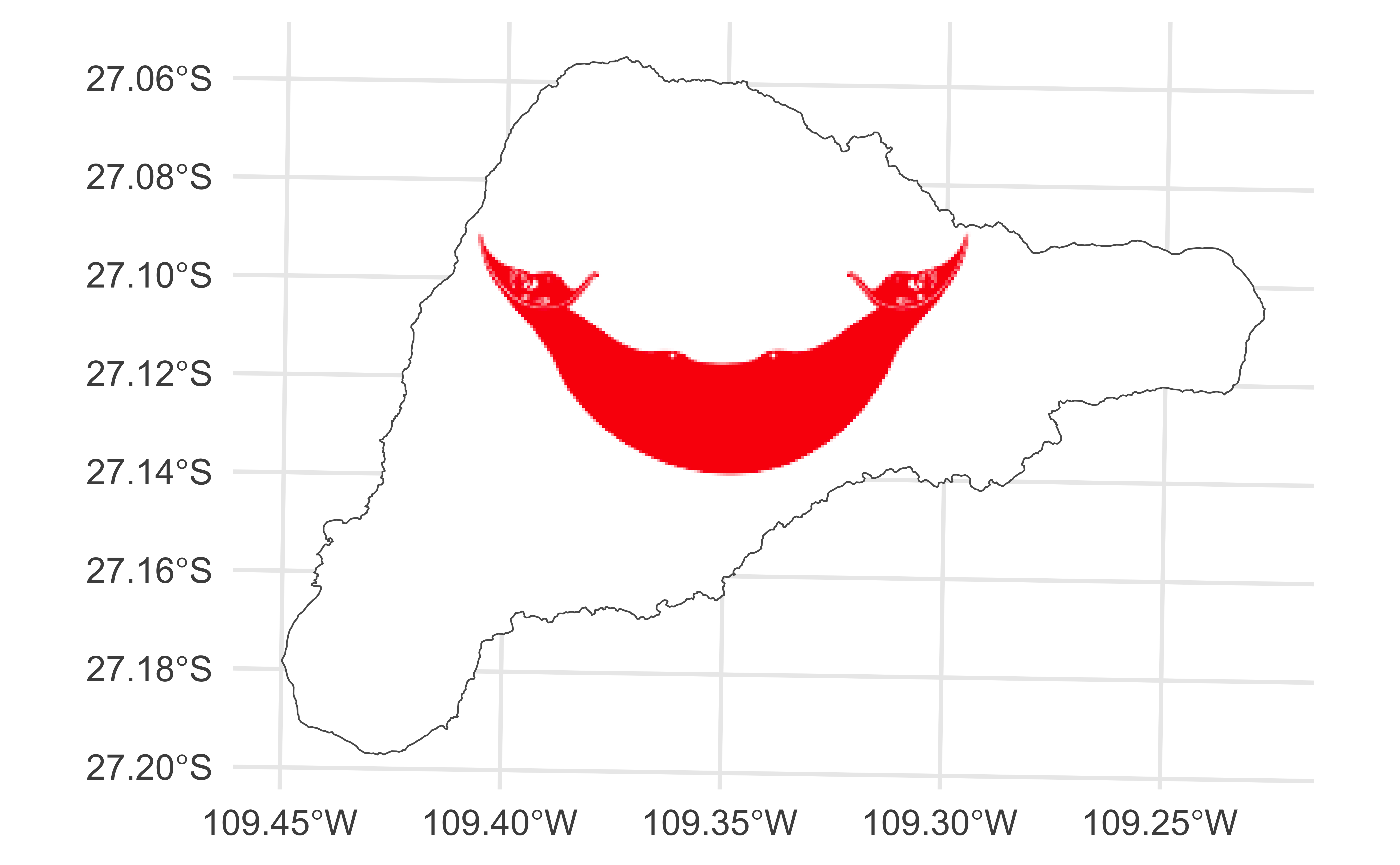
Layering with ggplot2

What are the layers in the following plot? What variables are being plotted?

Step 1

ggplot() +
  geom_sf(data = border)

Step 2

ggplot() +
  geom_sf(data = border) +
  geom_stars(data = elev)

Step 3

ggplot() +
  geom_sf(data = border) +
  geom_stars(data = elev) +
  scale_fill_distiller(name = "Elevation", palette = "RdYlGn", na.value = "transparent")

Step 4

ggplot() +
  geom_sf(data = border) +
  geom_stars(data = elev) +
  scale_fill_distiller(name = "Elevation", palette = "RdYlGn", na.value = "transparent") +
  geom_sf(data = roads, aes(linewidth = strokelwd))

Step 5

ggplot() +
  geom_sf(data = border) +
  geom_stars(data = elev) +
  scale_fill_distiller(name = "Elevation", palette = "RdYlGn", na.value = "transparent") +
  geom_sf(data = roads, aes(linewidth = strokelwd)) +
  scale_linewidth_continuous(range = c(0.1, 1))

Step 6

ggplot() +
  geom_sf(data = border) +
  geom_stars(data = elev) +
  scale_fill_distiller(name = "Elevation", palette = "RdYlGn", na.value = "transparent") +
  geom_sf(data = roads, aes(linewidth = strokelwd)) +
  scale_linewidth_continuous(range = c(0.1, 1)) +
  geom_sf(data = points, aes(fill = type), shape = 24, size = 3)

Error in `scale_fill_distiller()`:
! Discrete value supplied to a continuous scale.
ℹ Example values: "cave_entrance" and "volcano".

Step 6 - again

ggplot() +
  geom_sf(data = border) +
  geom_stars(data = elev) +
  scale_fill_distiller(name = "Elevation", palette = "RdYlGn", na.value = "transparent") +
  geom_sf(data = roads, aes(linewidth = strokelwd)) +
  scale_linewidth_continuous(range = c(0.1, 1)) +
  new_scale_fill() +
  geom_sf(data = points, aes(fill = type), shape = 24, size = 3)

Step 7

ggplot() +
  geom_sf(data = border) +
  geom_stars(data = elev) +
  scale_fill_distiller(name = "Elevation", palette = "RdYlGn", na.value = "transparent") +
  geom_sf(data = roads, aes(linewidth = strokelwd)) +
  scale_linewidth_continuous(range = c(0.1, 1)) +
  new_scale_fill() +
  geom_sf(data = points, aes(fill = type), shape = 24, size = 3) +
  scale_fill_manual(name = "Type", values = c("gray50", "gold", "firebrick3"))

Step 8

ggplot() +
  geom_sf(data = border) +
  geom_stars(data = elev) +
  scale_fill_distiller(name = "Elevation", palette = "RdYlGn", na.value = "transparent") +
  geom_sf(data = roads, aes(linewidth = strokelwd)) +
  scale_linewidth_continuous(range = c(0.1, 1)) +
  new_scale_fill() +
  geom_sf(data = points, aes(fill = type), shape = 24, size = 3) +
  scale_fill_manual(name = "Type", values = c("gray50", "gold", "firebrick3")) +
  guides(linewidth = "none") +
  labs(x = NULL, y = NULL)

Step 8