# load packages
library(tidyverse)
library(tidymodels)
library(openintro)
library(scales)
library(ggrepel)
library(colorspace)
library(ggthemes)
library(paletteer)

# set theme for ggplot2
ggplot2::theme_set(ggplot2::theme_minimal(base_size = 16))

# set figure parameters for knitr
knitr::opts_chunk$set(
  fig.width = 7, # 7" width
  fig.asp = 0.618, # the golden ratio
  fig.retina = 3, # dpi multiplier for displaying HTML output on retina
  fig.align = "center", # center align figures
  dpi = 300 # higher dpi, sharper image
)Colors
Lecture 14
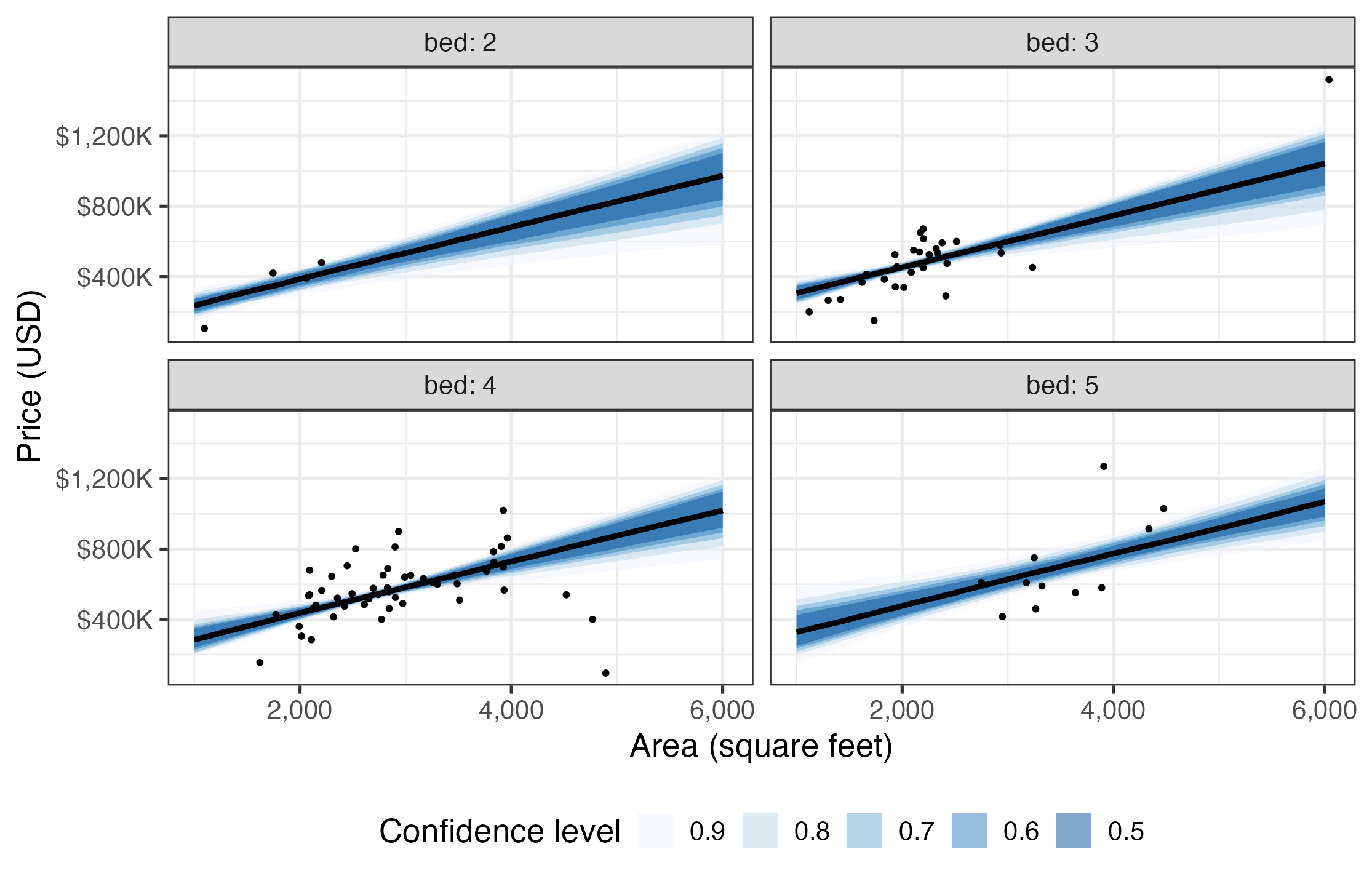
ae-09: Part 1
The following visualization shows bootstrap confidence intervals for predictions from additive (main effects) models for predicting price from area and number of bedrooms. Recreate the visualization.
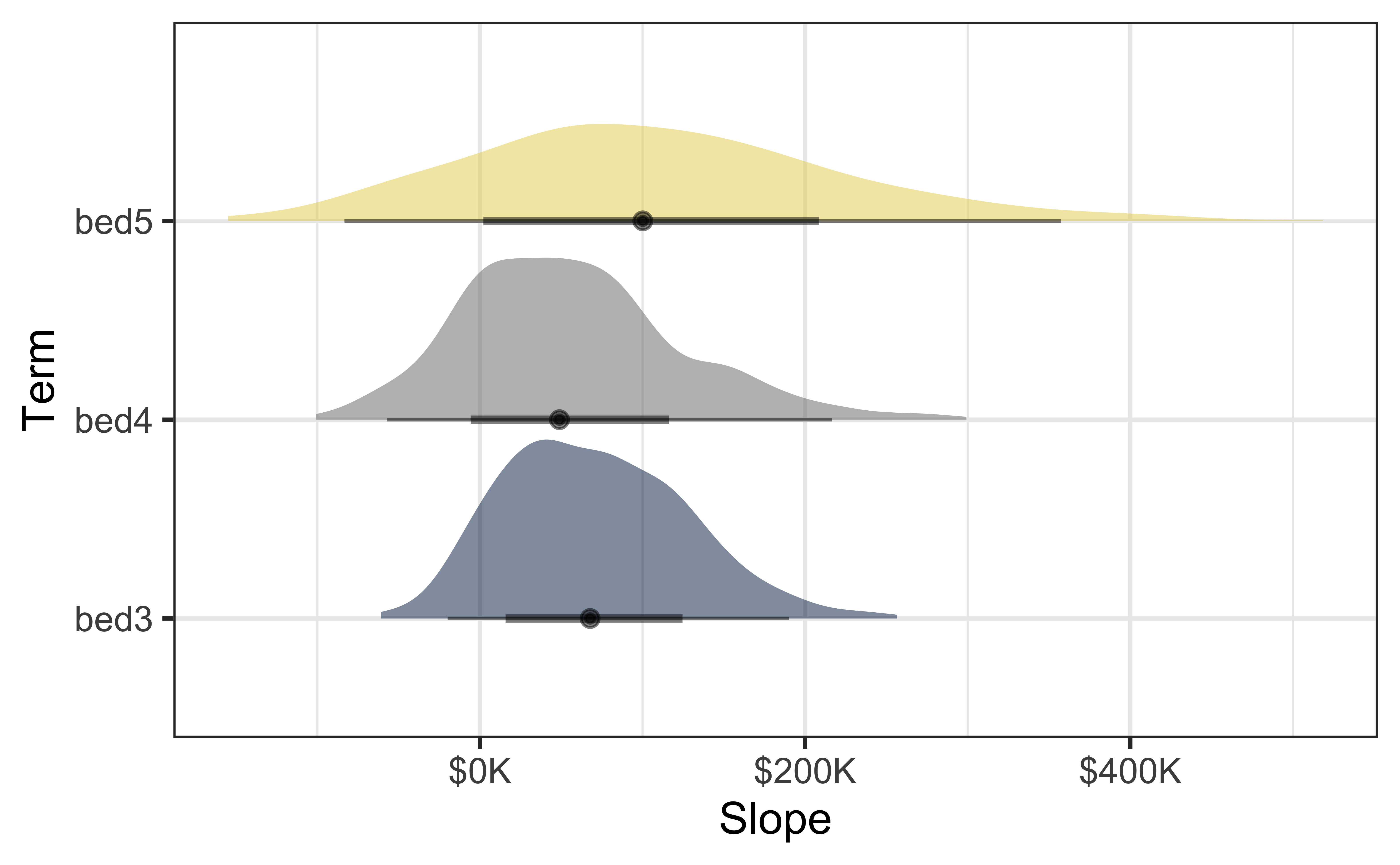
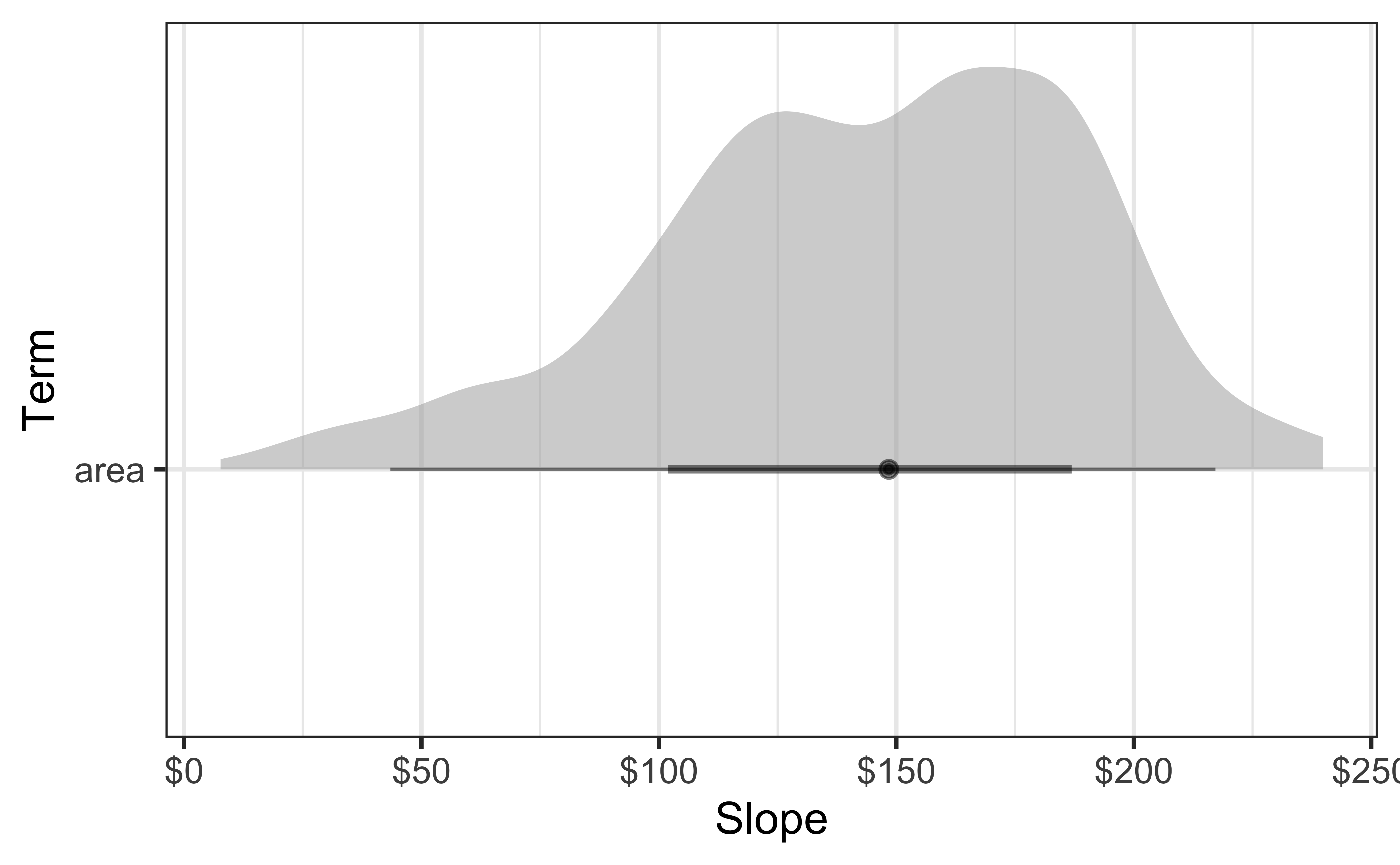
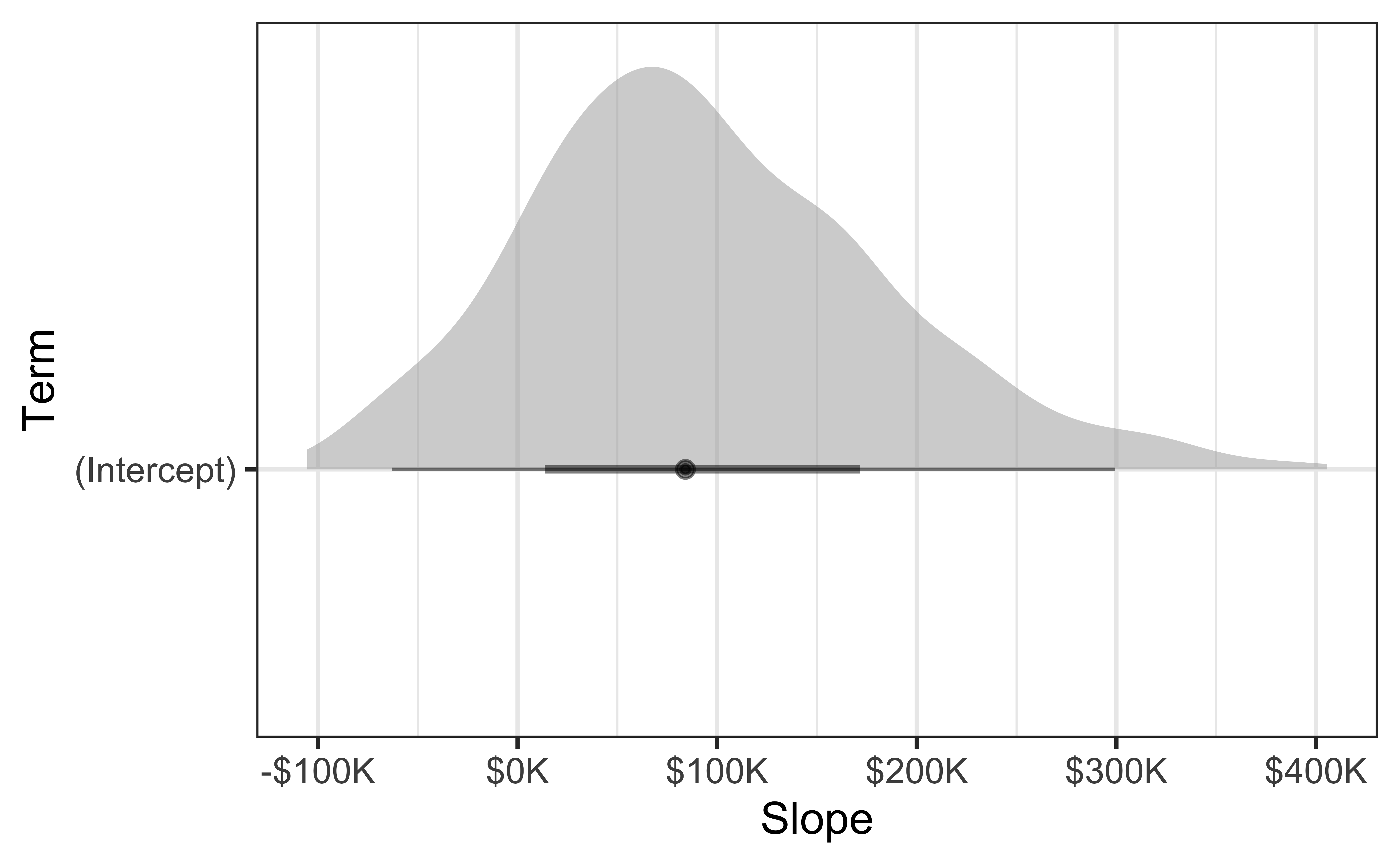
ae-09: Part 2
Construct and visualize bootstrap distributions of model estimates using halfeye plots, i.e., recreate the following visualization. Then, try other stats (other ways of visualizing the distributions) from the ggdist package.
Uses of color in data visualization
- Distinguish categories (qualitative)

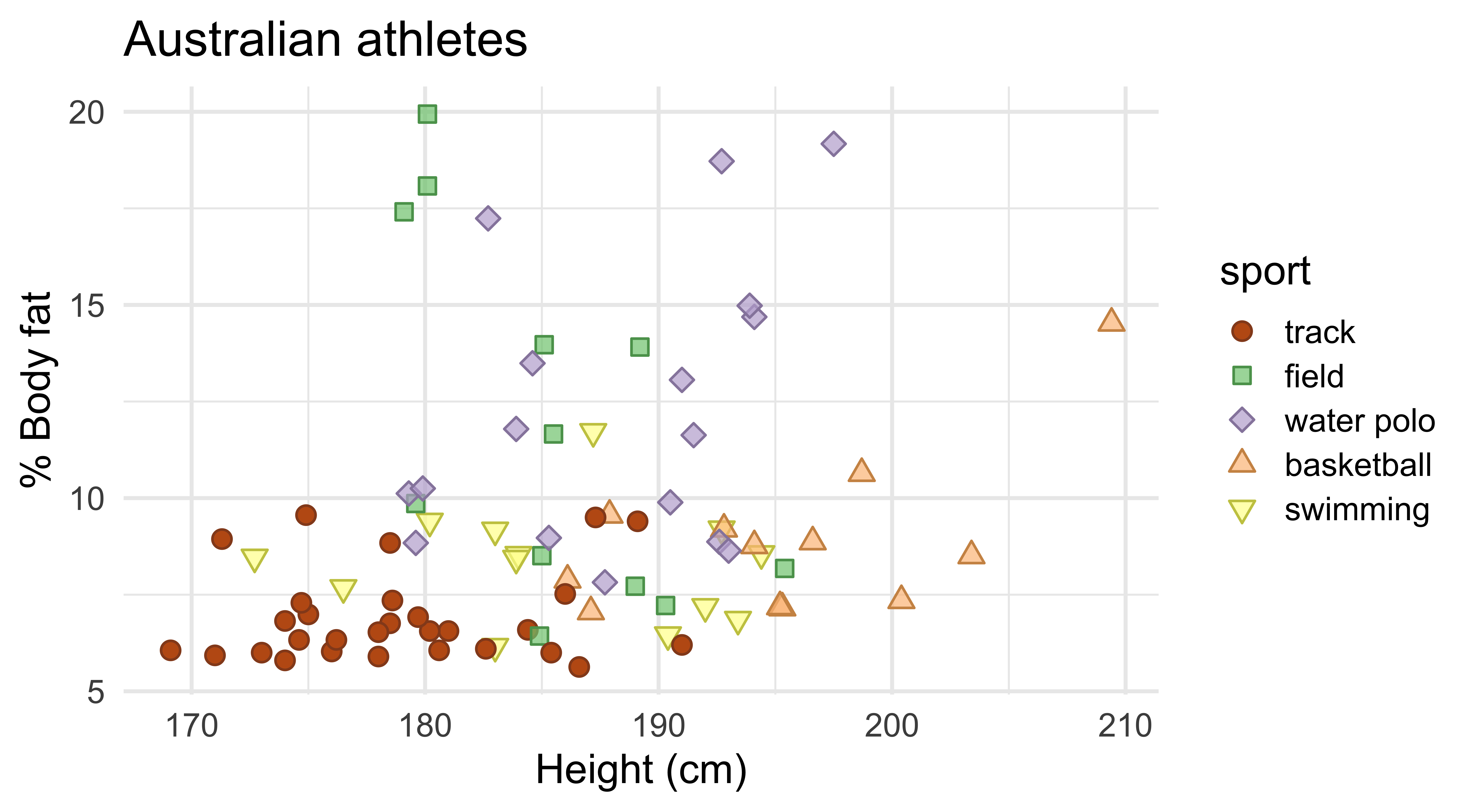
Qualitative scale: Okabe-Ito palette
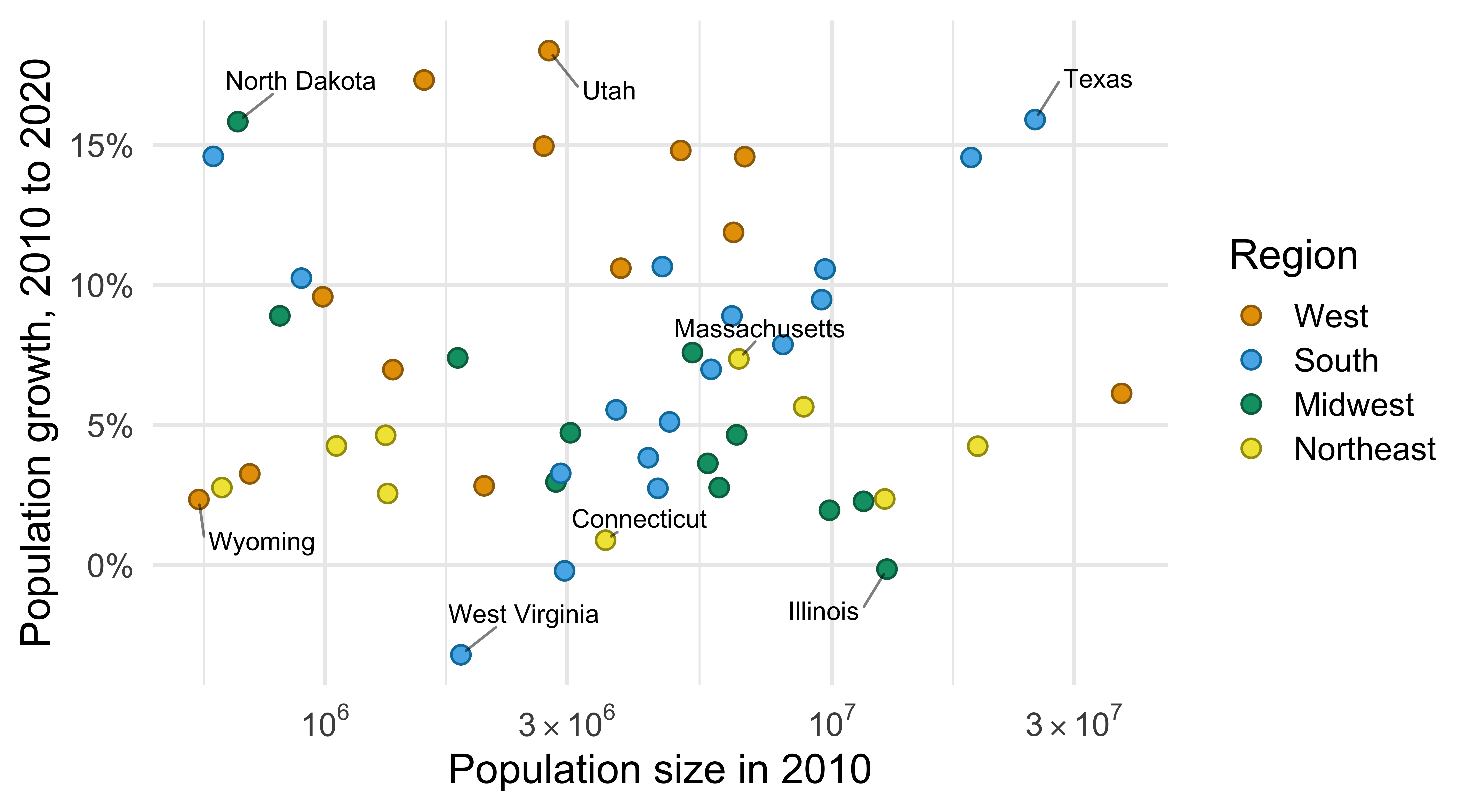
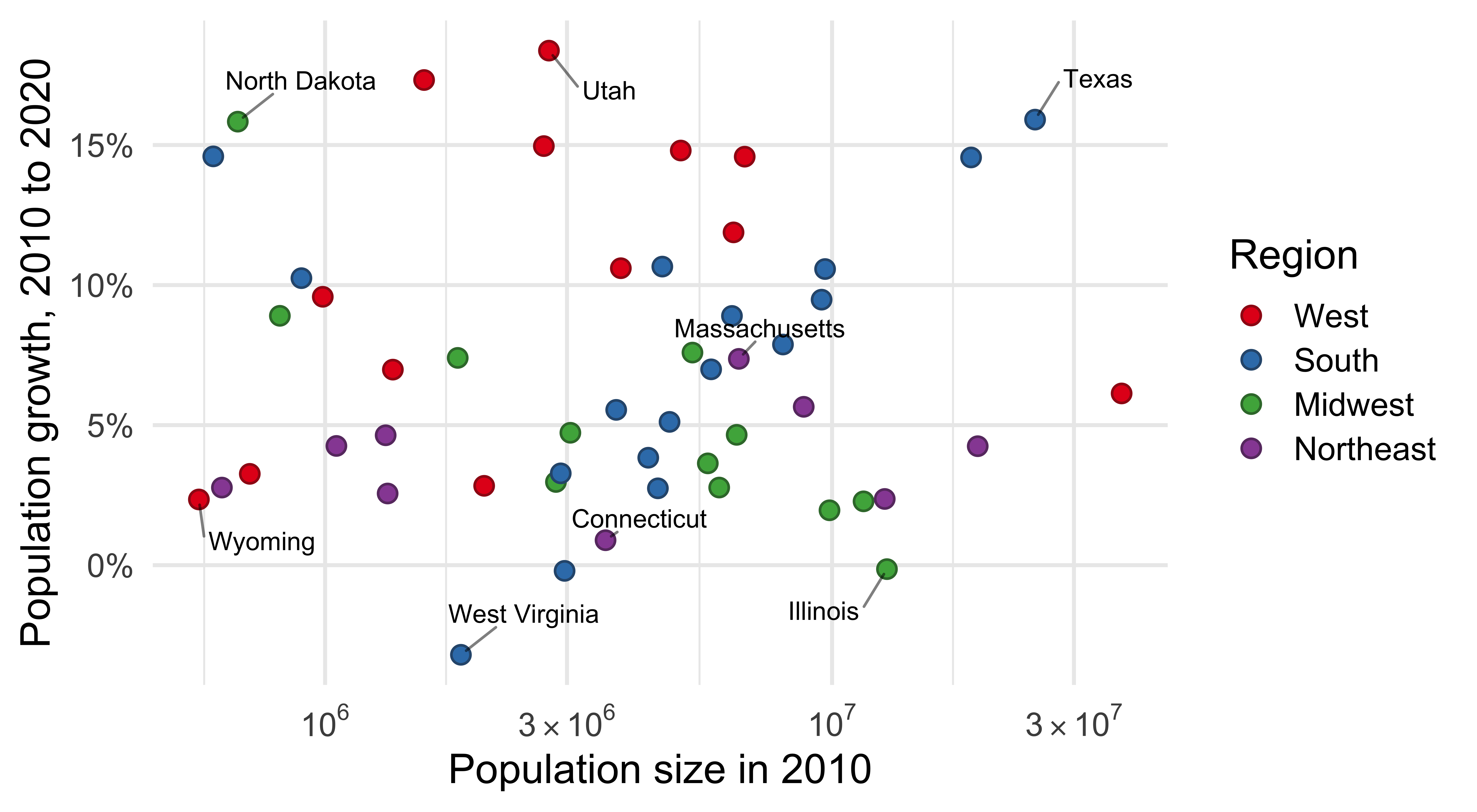
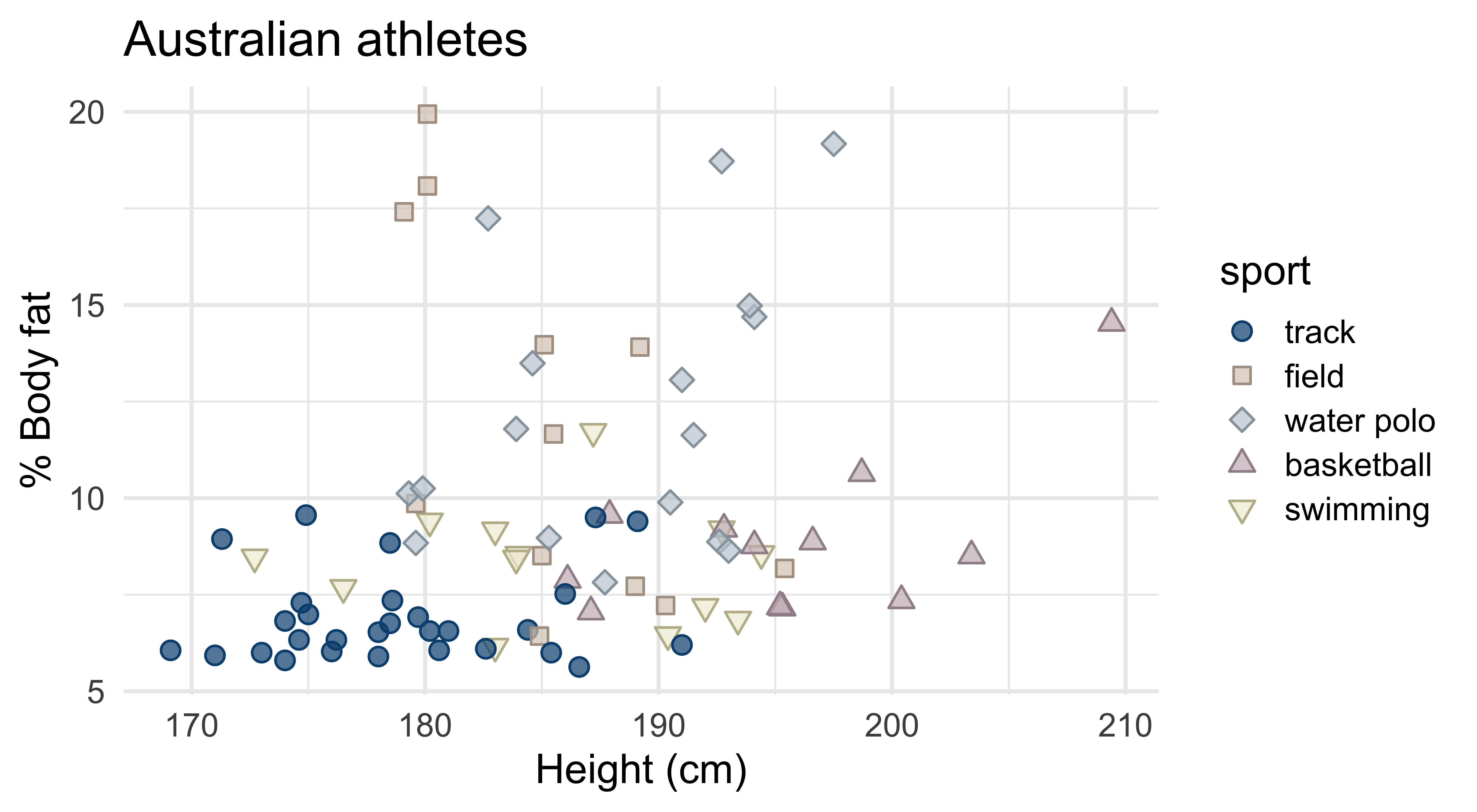
Qualitative scale: ColorBrewer Set1
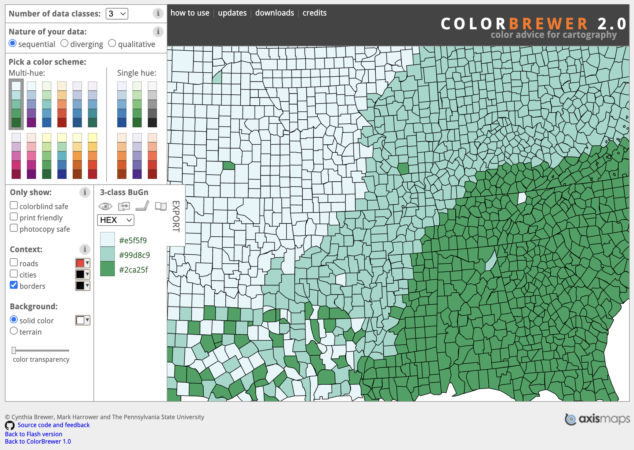
Aside: ColorBrewer
ColorBrewer is an online tool developed in 2002 for selecting thematic map color schemes based on Dr. Cynthia Brewer’s palettes.
Qualitative scale: ColorBrewer Set3
Uses of color in data visualization
- Distinguish categories (qualitative)
- Represent numeric values (sequential)

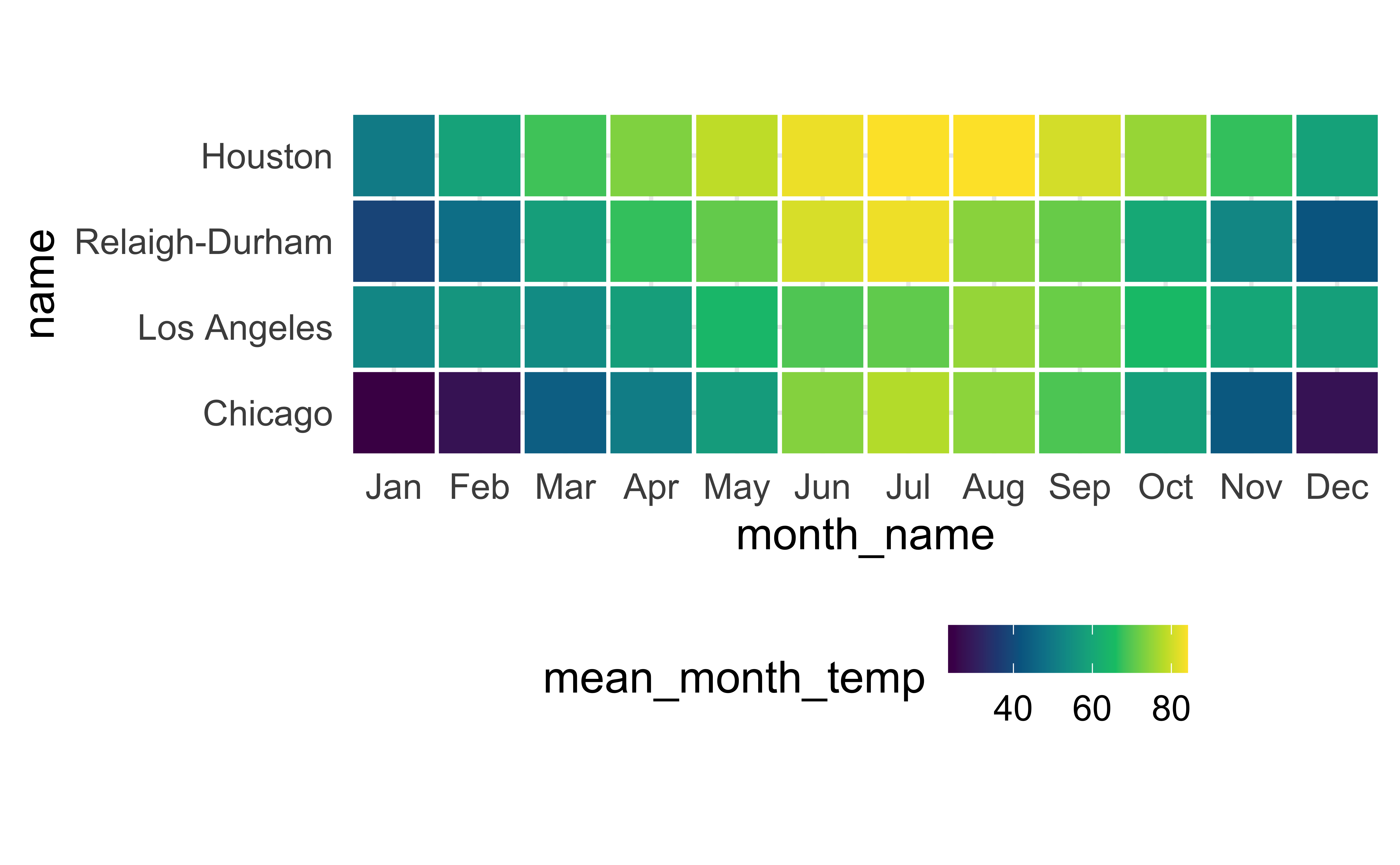
Sequential scale: Viridis palette
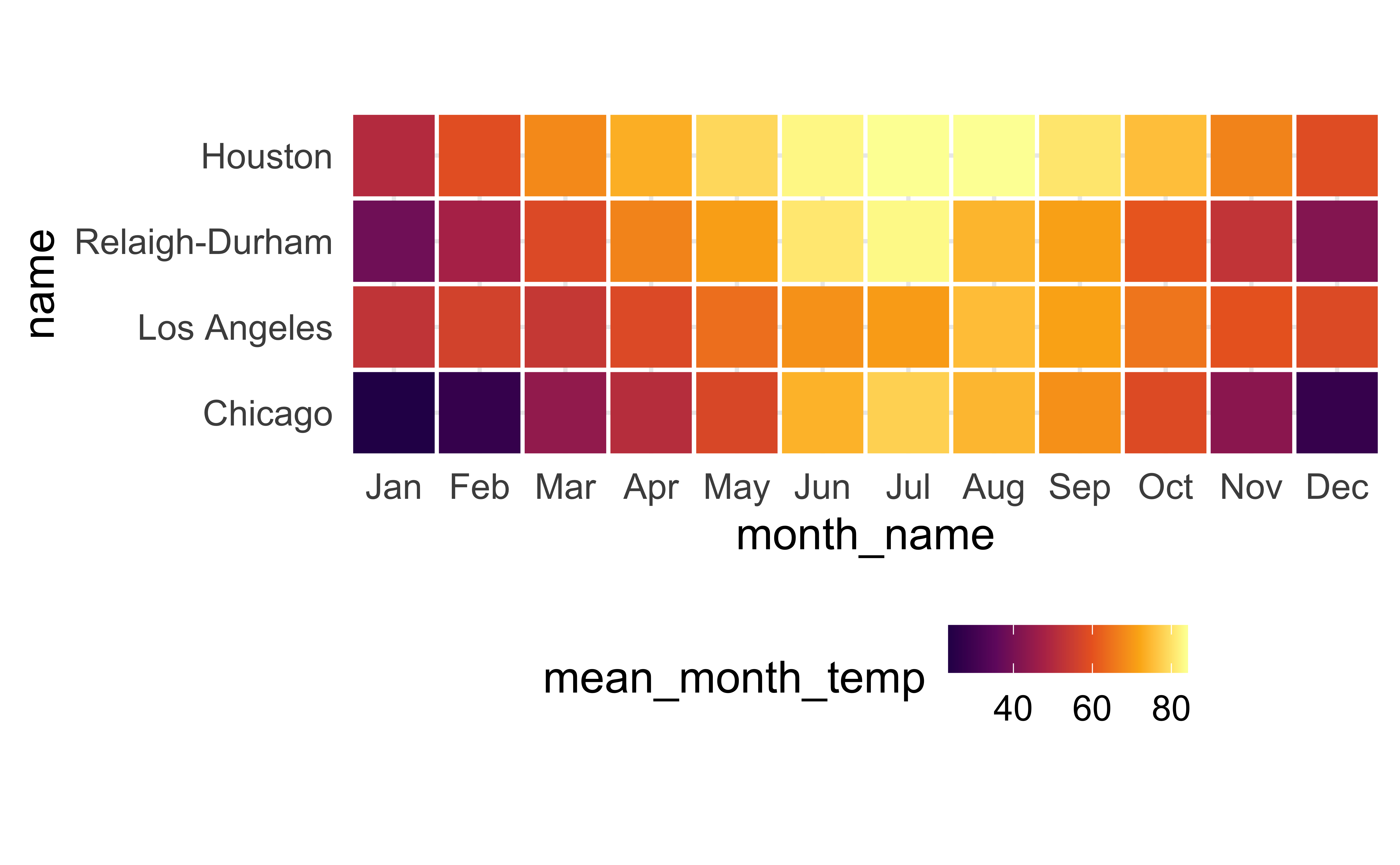
Sequential scale: Inferno palette
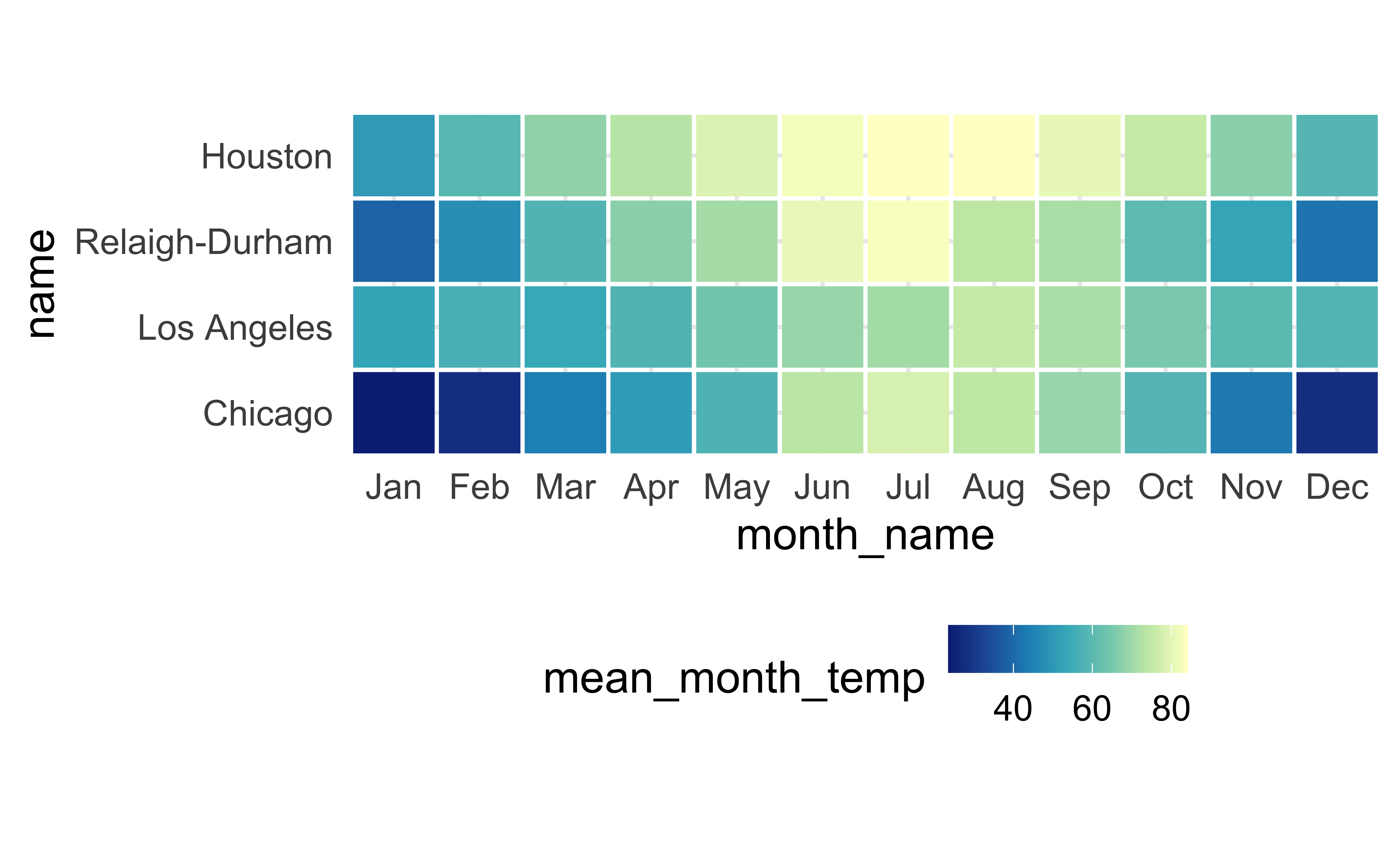
Sequential scale: Cividis palette
Uses of color in data visualization
- Distinguish categories (qualitative)
- Represent numeric values (sequential)
- Represent numeric values (diverging)

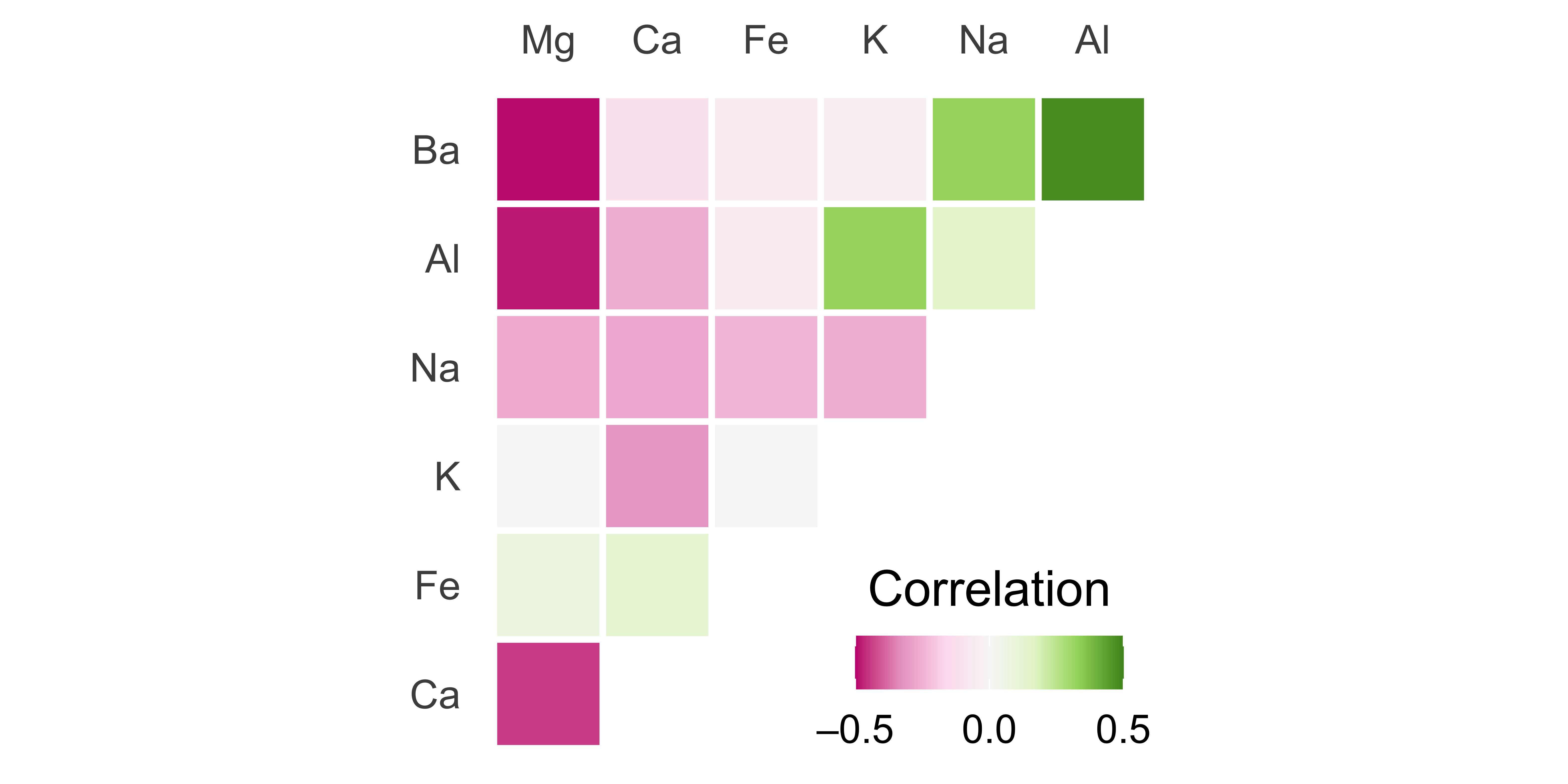
Diverging scale: ColorBrewer PiYG palette
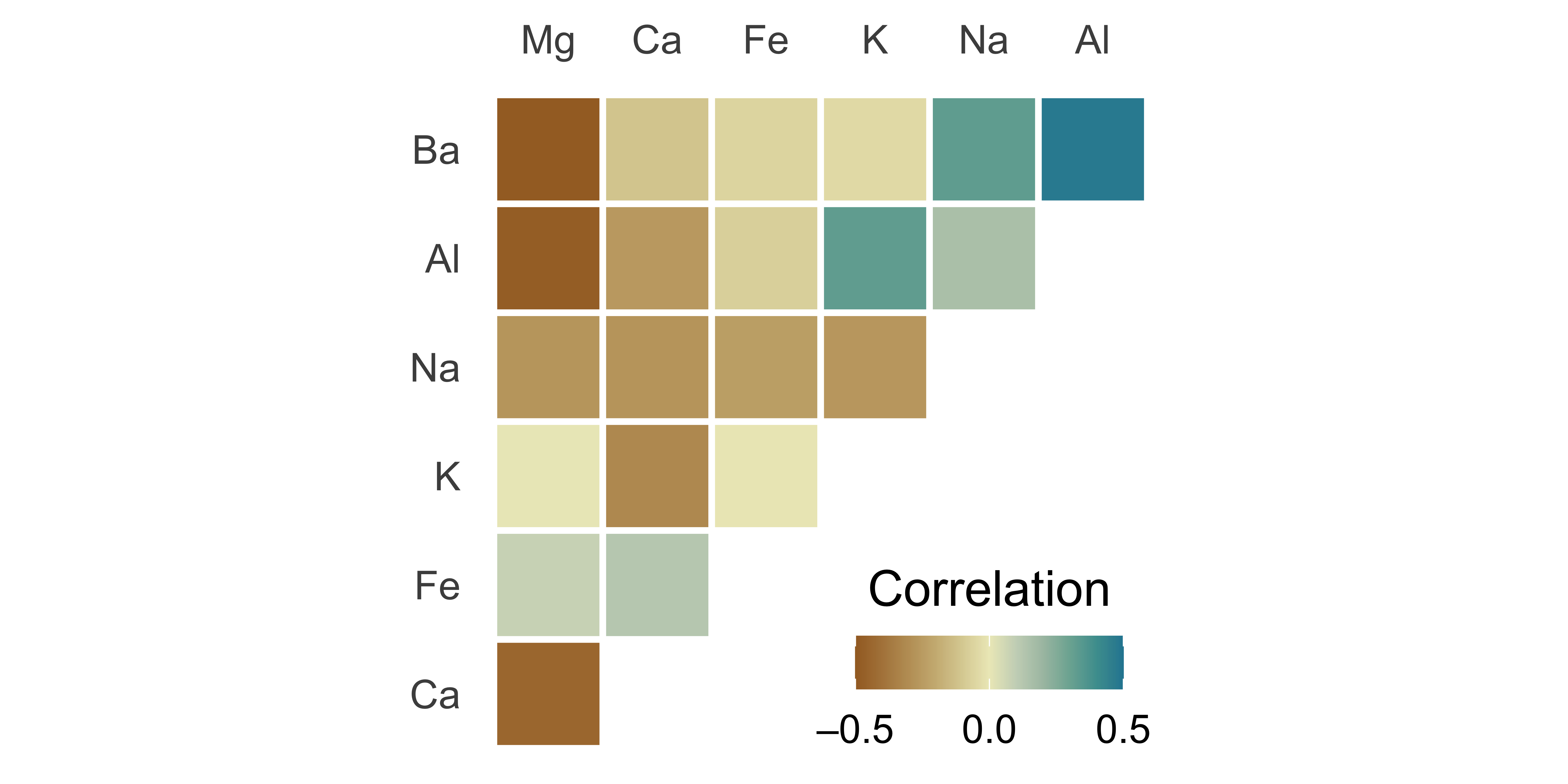
Diverging scale: ColorBrewer CartoEarth palette
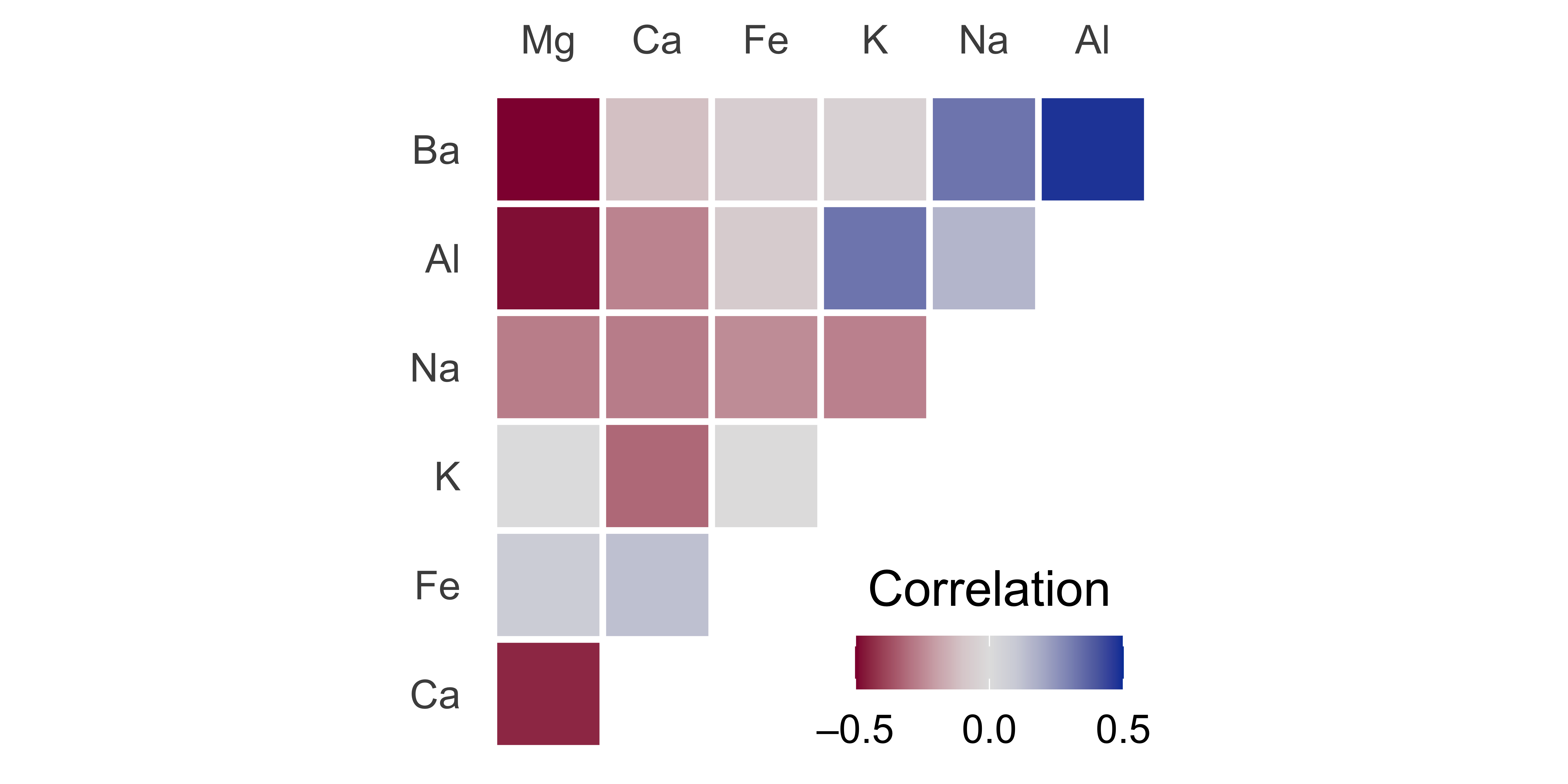
Diverging scale: Blue-Red palette
Uses of color in data visualization
- Distinguish categories (qualitative)
- Represent numeric values (sequential)
- Represent numeric values (diverging)
- Highlight

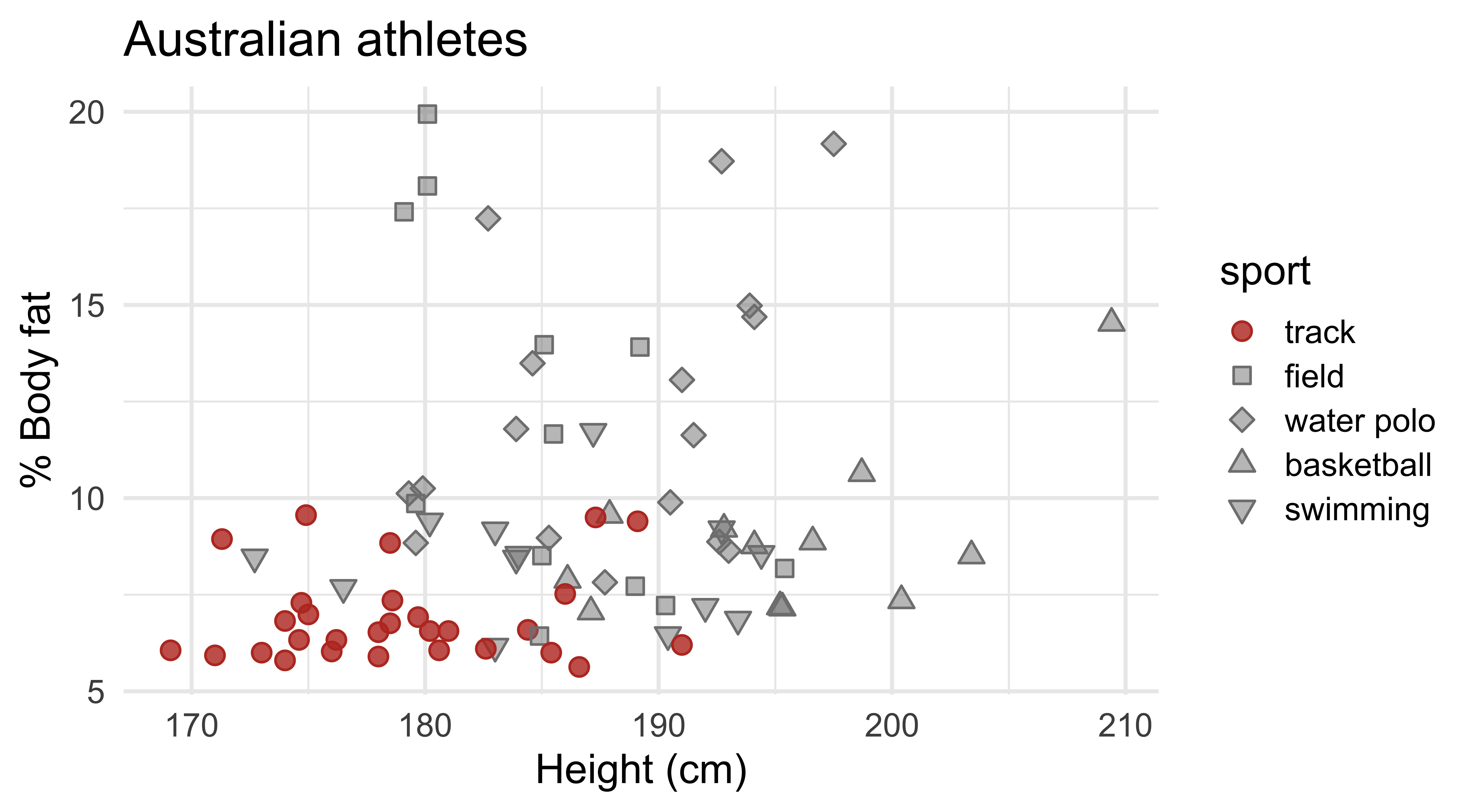
Highlighting: Grays with accents
Highlighting: Okabe-Ito accent
Highlighting: ColorBrewer accent
Uses of color in data visualization
- Distinguish categories (qualitative)
- Represent numeric values (sequential)
- Represent numeric values (diverging)
- Highlight
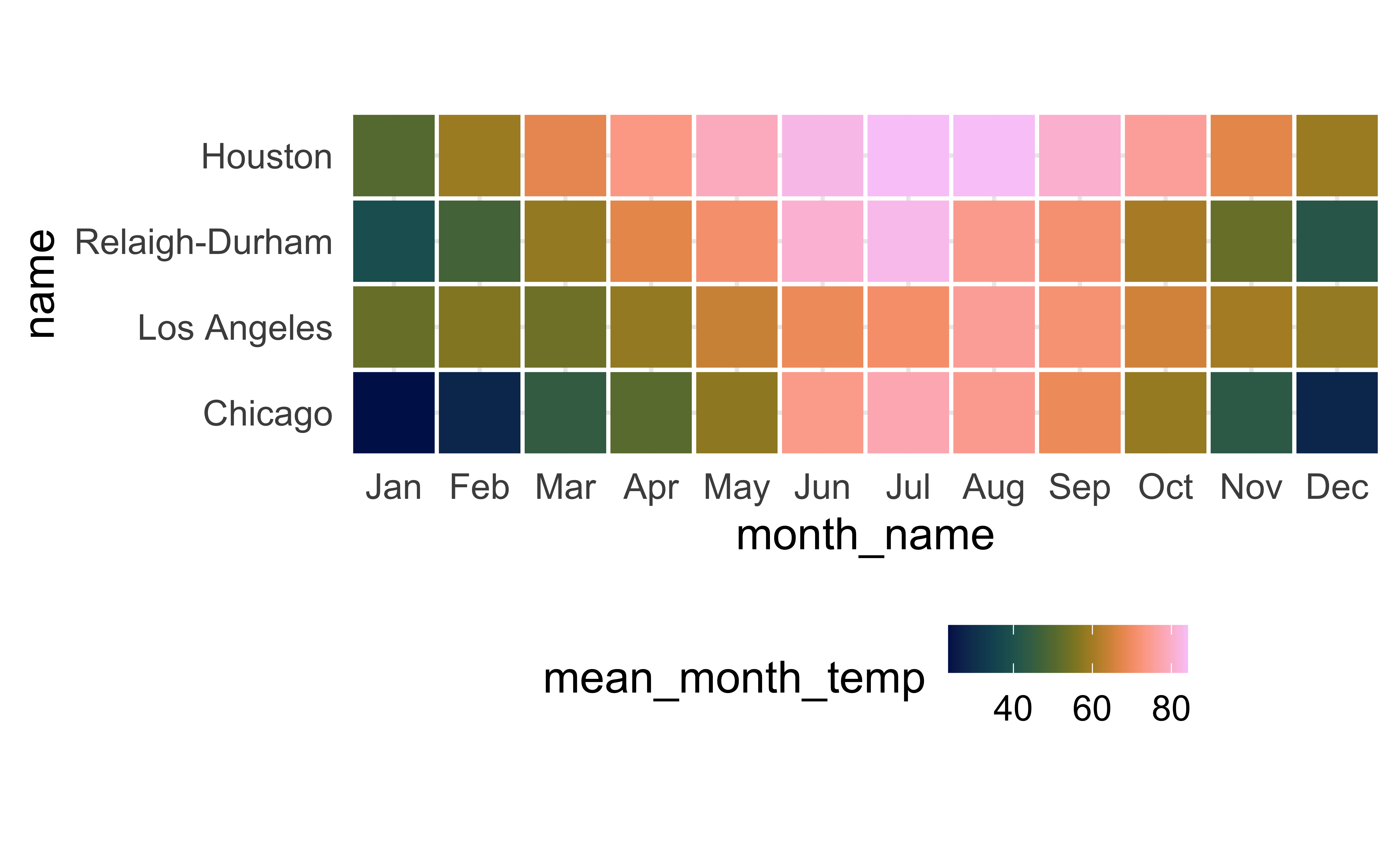
Default scale
No fill scale defined, default is scale_fill_gradient():

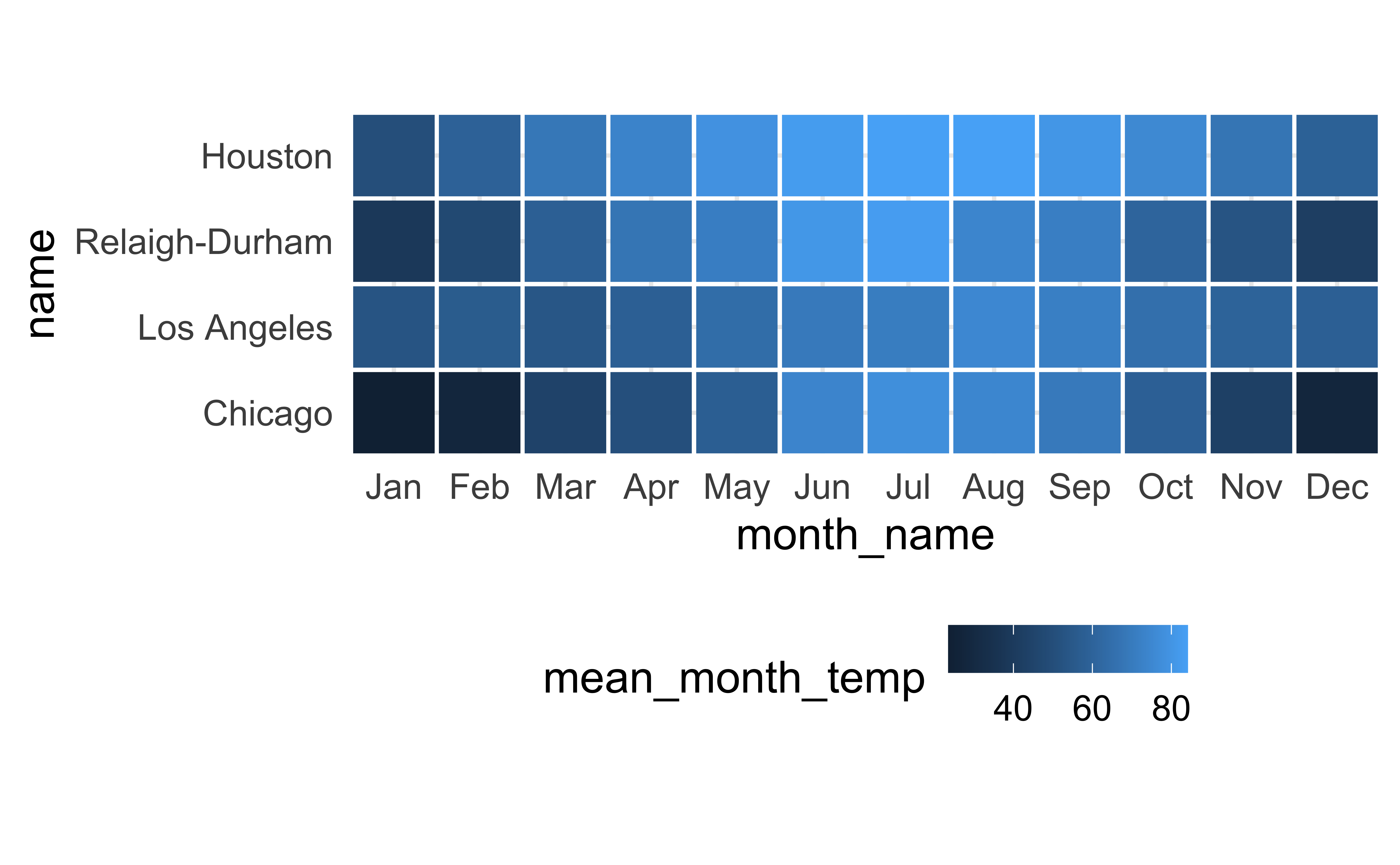
scale_fill_gradient()
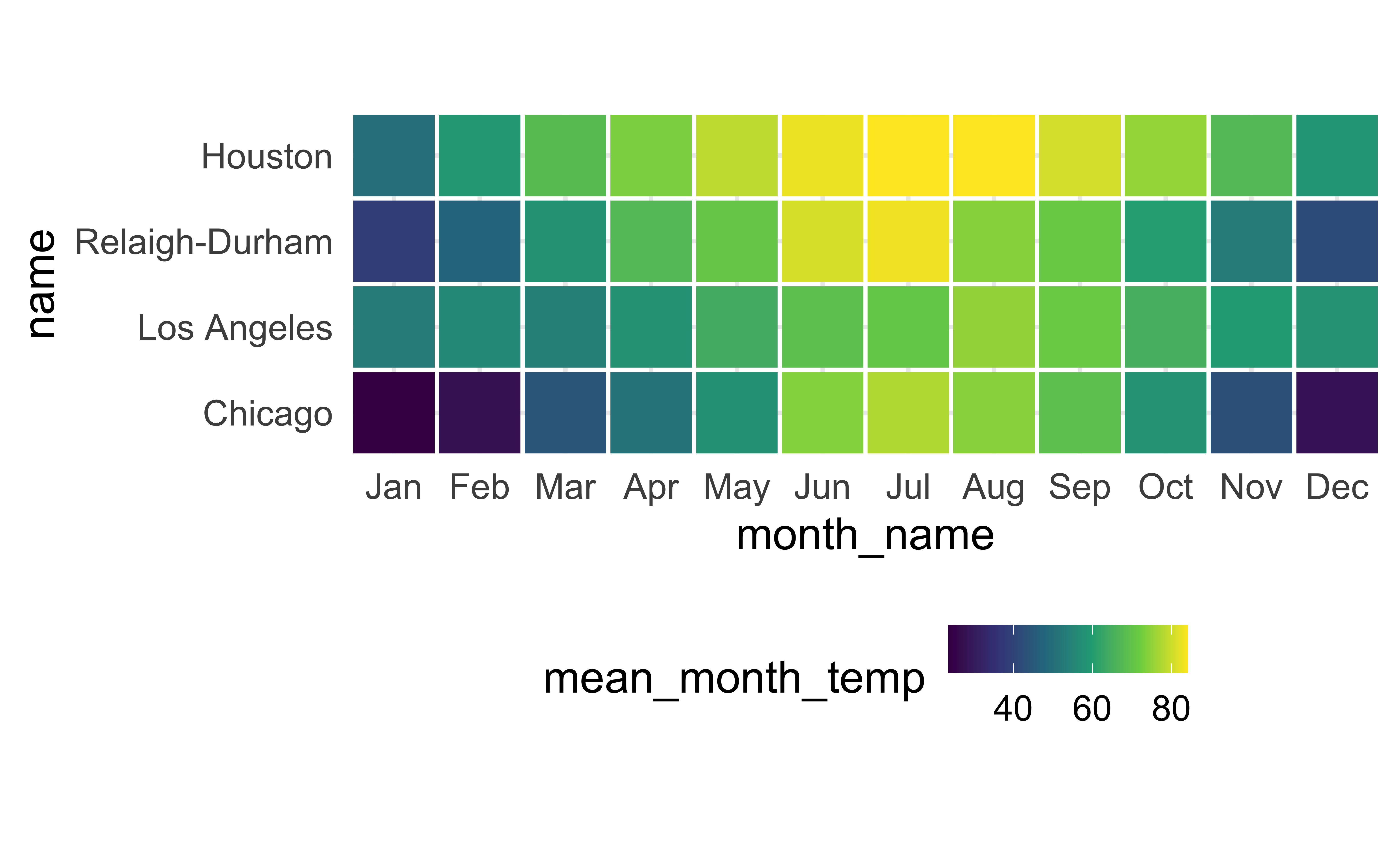
scale_fill_viridis_c()
Viridis palette options
scale_fill_distiller()
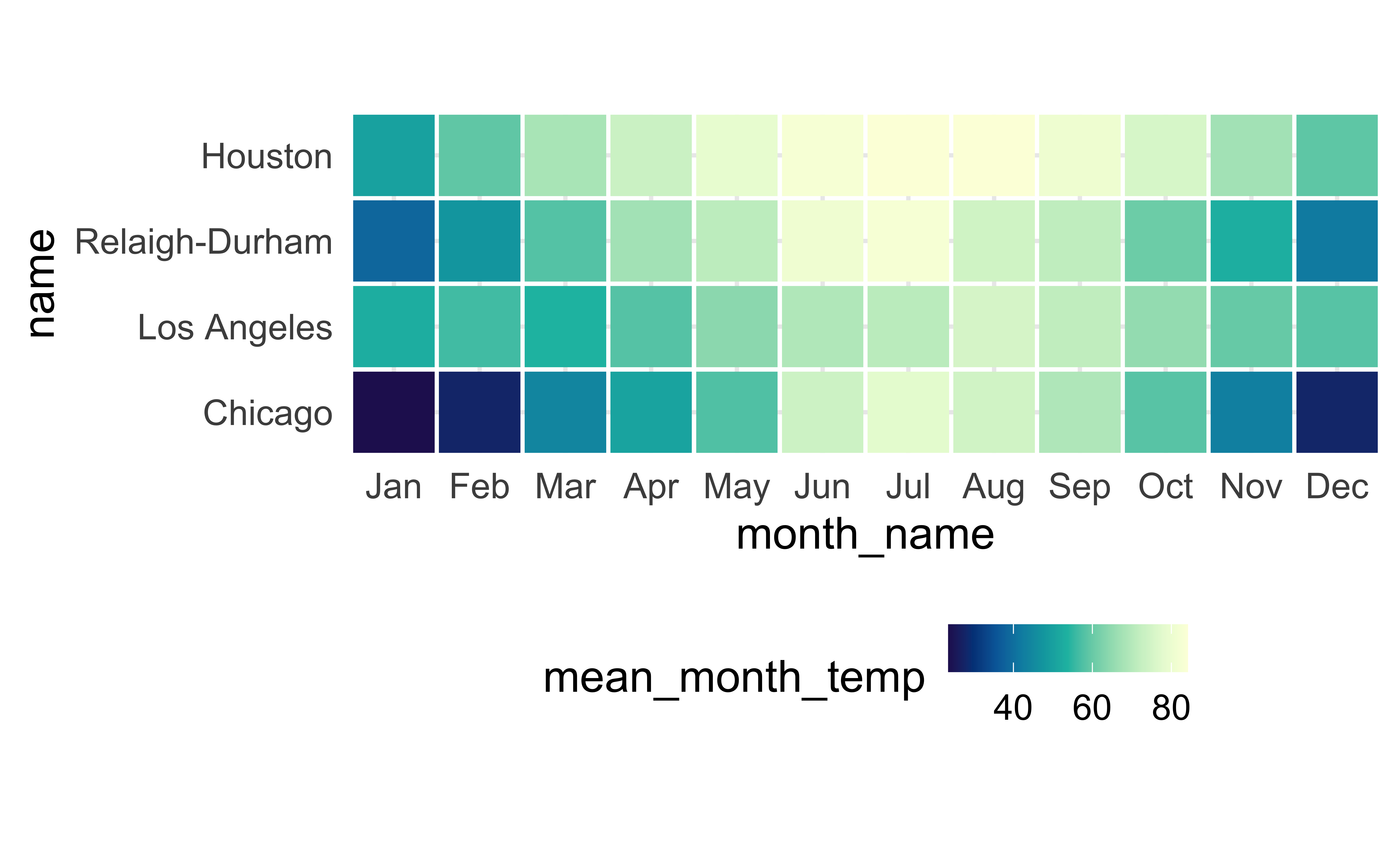
scale_fill_continuous_sequential() + Multi-hue
scale_fill_continuous_sequential() + Viridis
scale_fill_continuous_sequential() + Inferno
HCL palettes: Sequential
HCL: Hue-Chroma-Luminance
HCL palettes: Diverging
HCL palettes: Divergingx
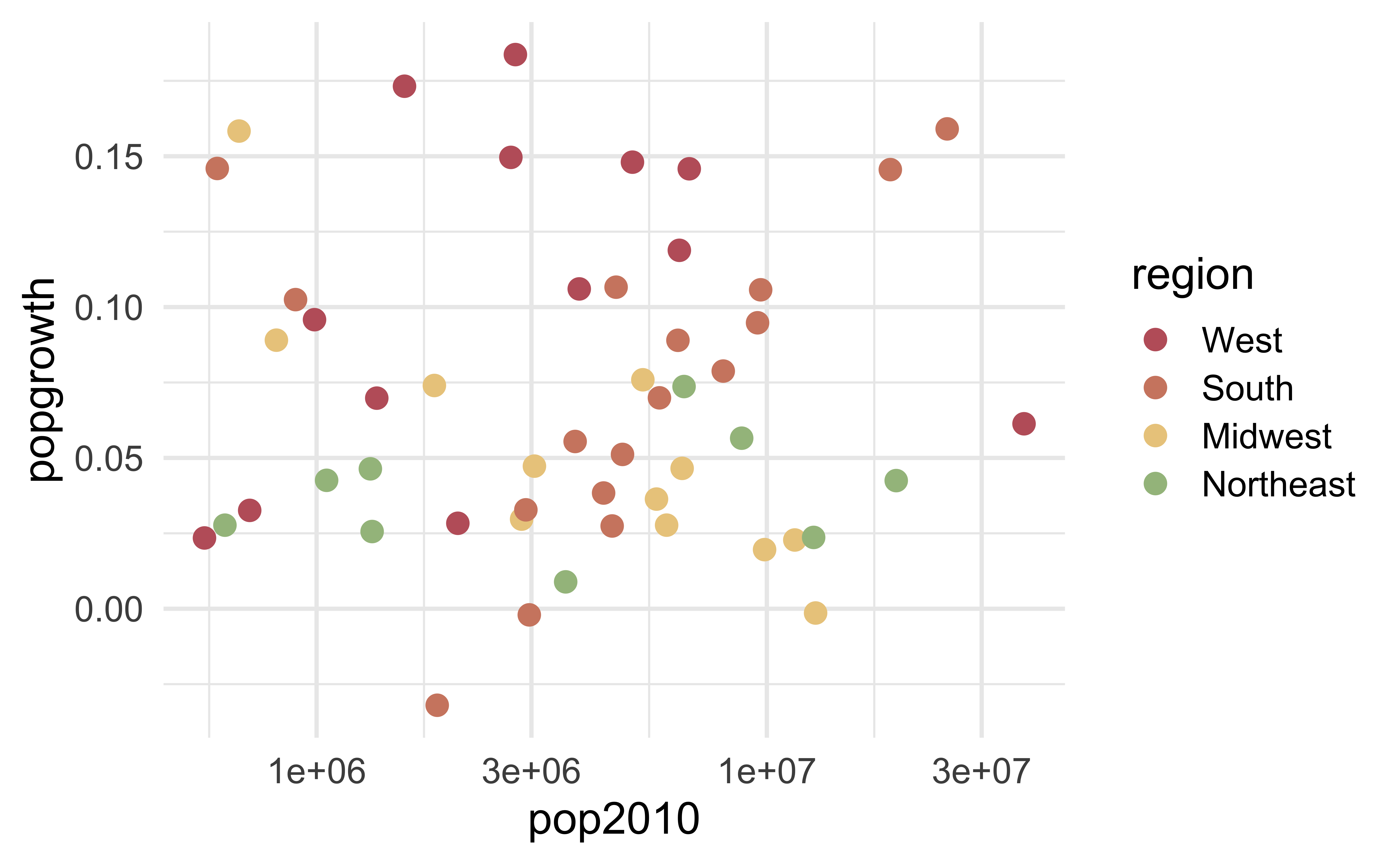
Default discrete scale
No color scale defined, default is scale_color_hue():
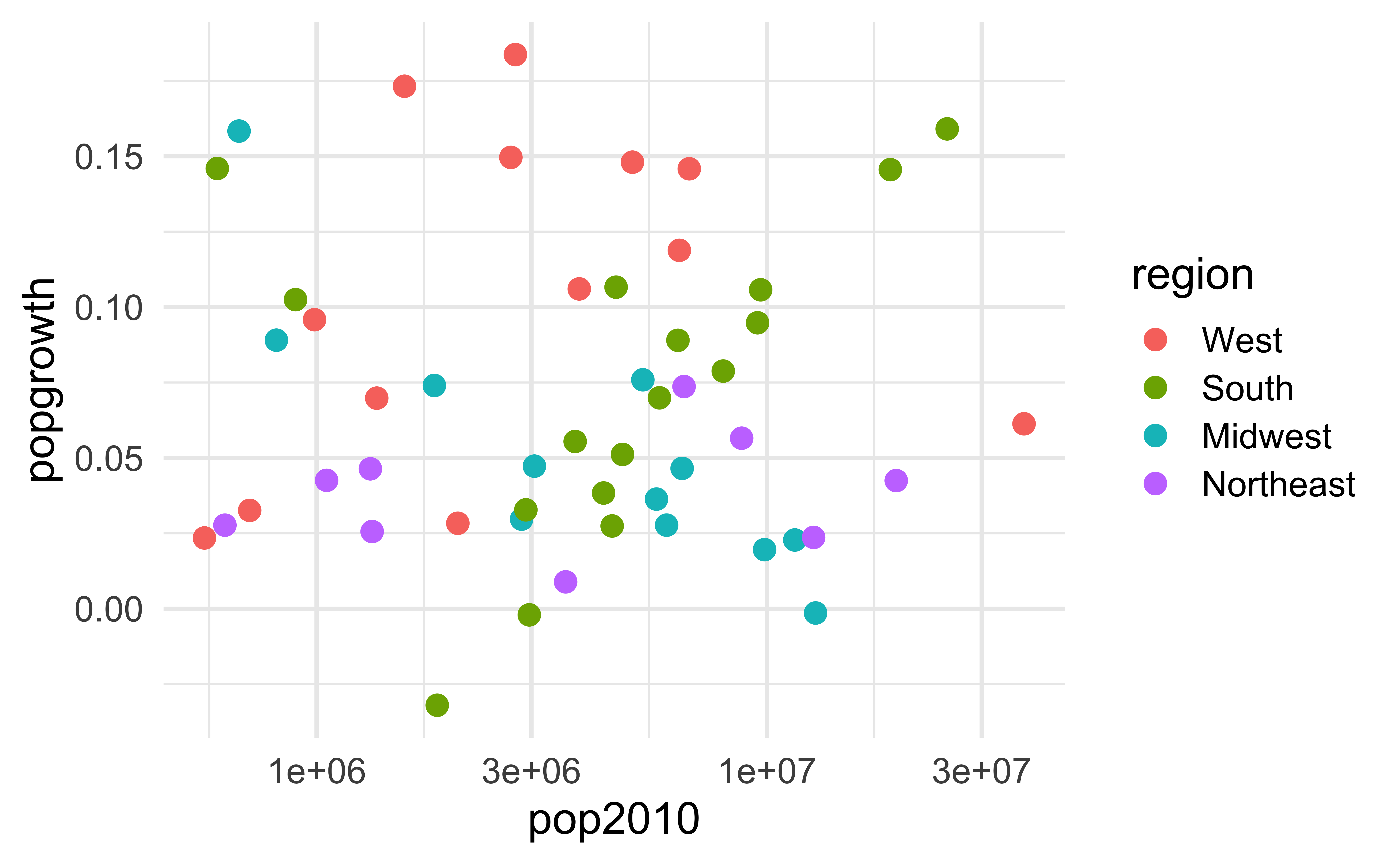
scale_color_hue()

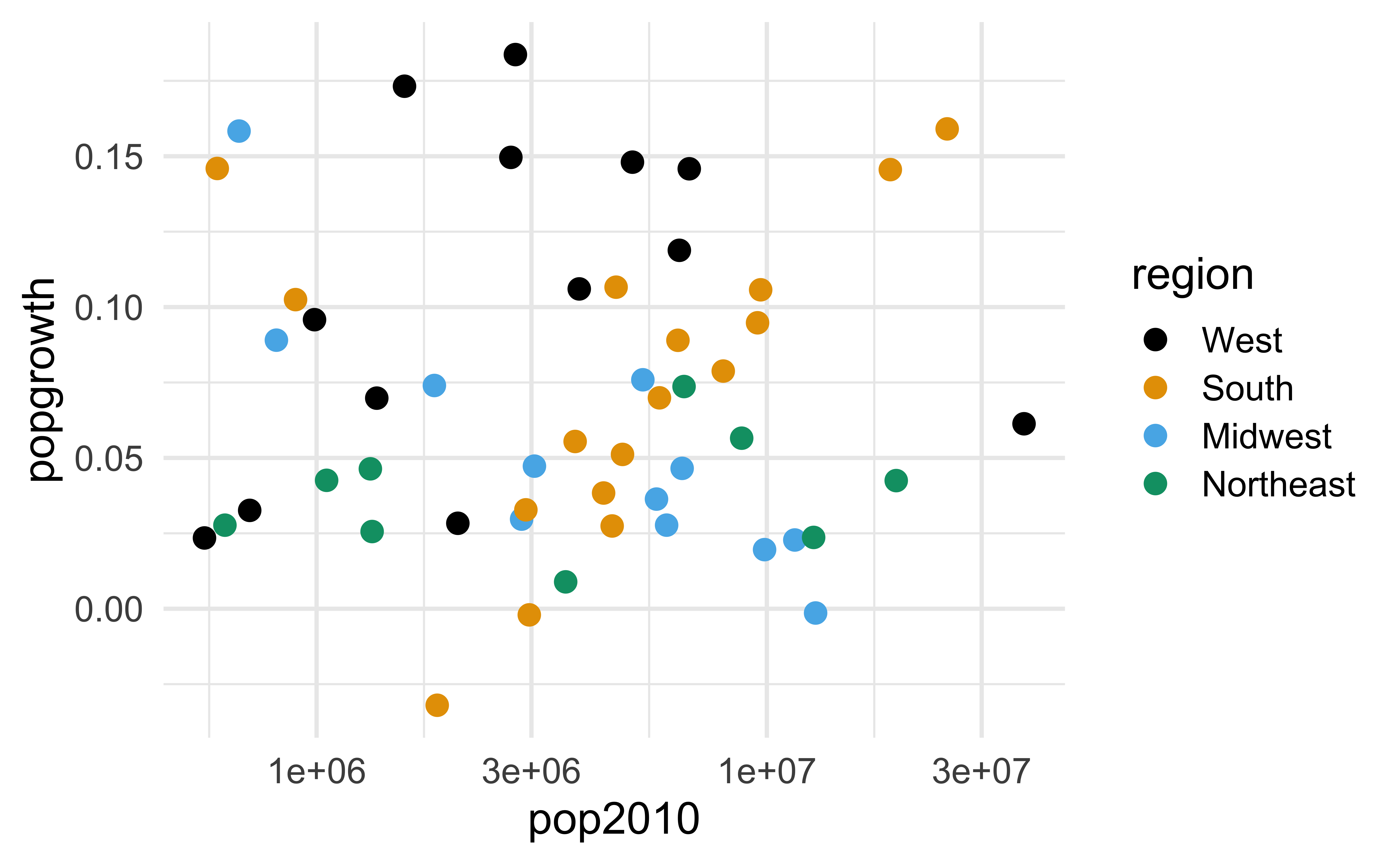
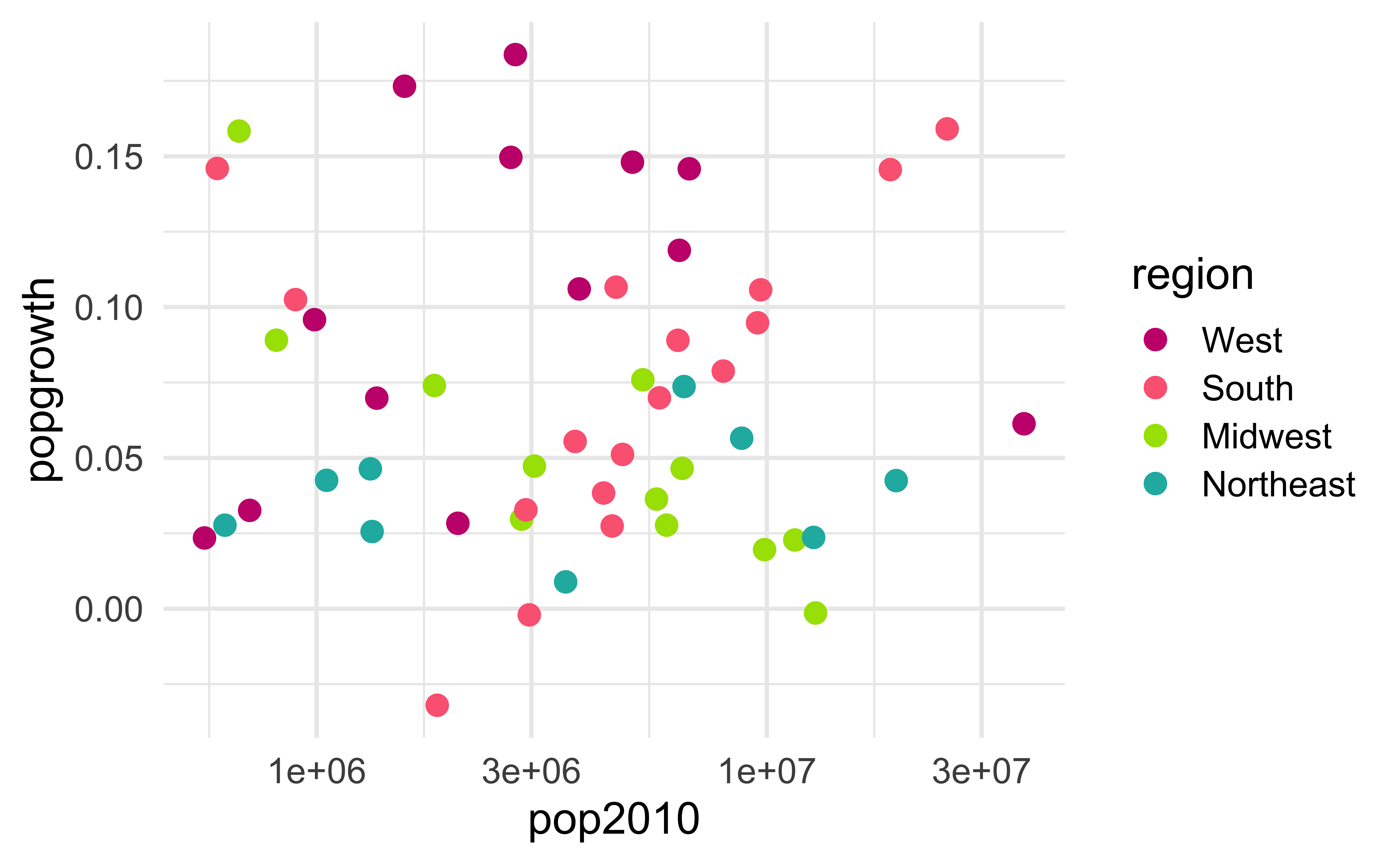
scale_color_colorblind()
Uses Okabe-Ito colors:
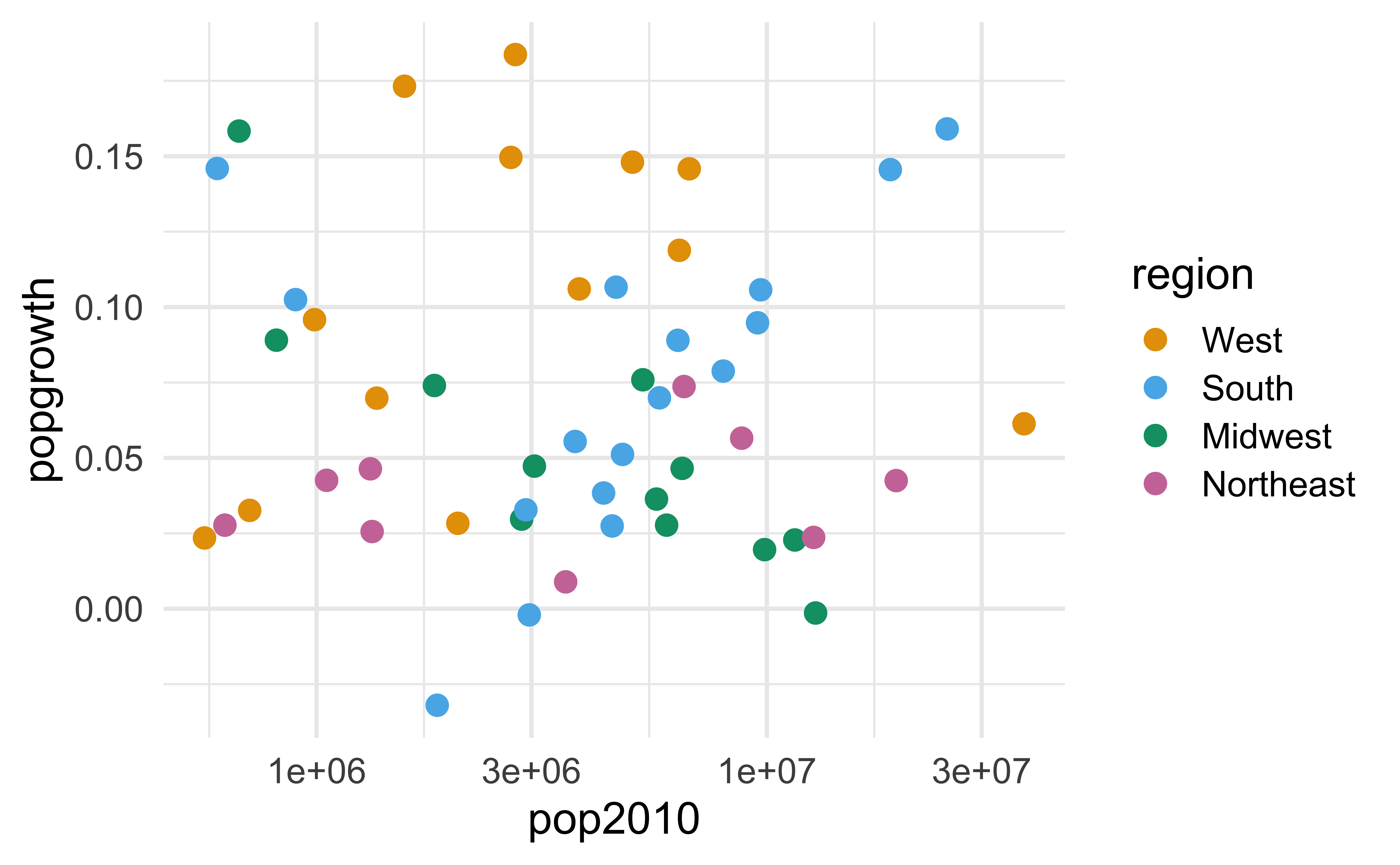
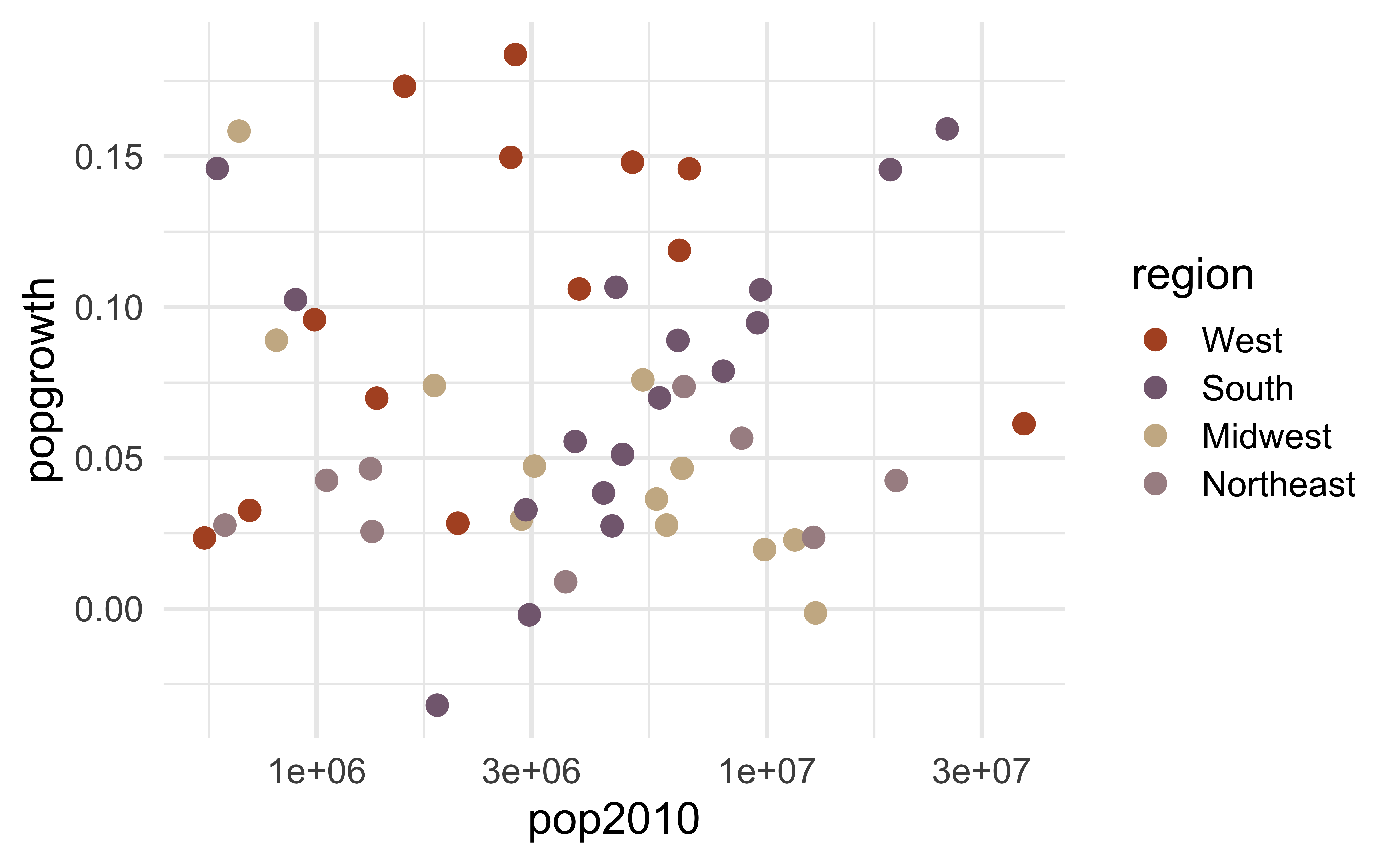
scale_color_manual()
Qualitative scales are best set manually:
Okabe-Ito RGB codes
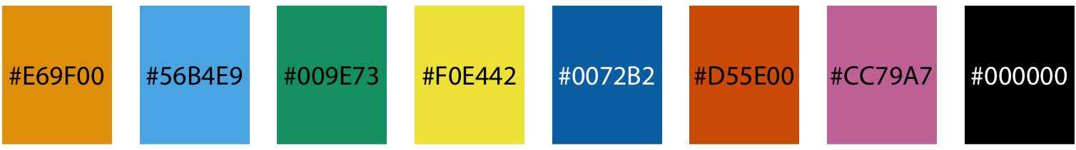
| Name | Hex code | R, G, B (0-255) |
|---|---|---|
| orange | #E69F00 | 230, 159, 0 |
| sky blue | #56B4E9 | 86, 180, 233 |
| bluish green | #009E73 | 0, 158, 115 |
| yellow | #F0E442 | 240, 228, 66 |
| blue | #0072B2 | 0, 114, 178 |
| vermilion | #D55E00 | 213, 94, 0 |
| reddish purple | #CC79A7 | 204, 121, 167 |
| black | #000000 | 0, 0, 0 |
palateeer + nord::aurora
https://github.com/jkaupp/nord
palateeer + LaCroixColoR::PassionFruit
https://github.com/johannesbjork/LaCroixColoR
palateeer + tayloRswift::taylor1989
https://asteves.github.io/tayloRswift/
palateeer + scico::lajolla
https://github.com/thomasp85/scico
5. Avoid high chroma
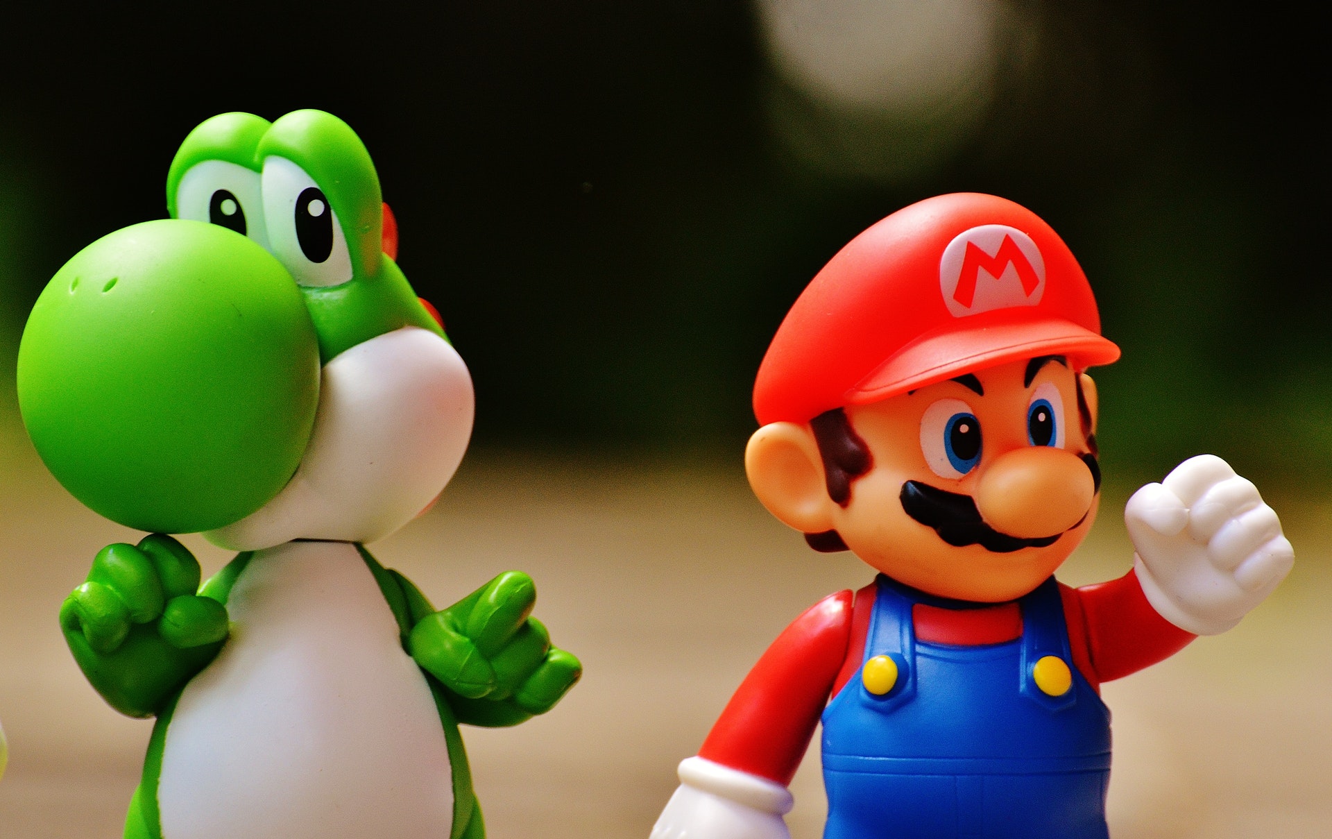
High chroma: Toys
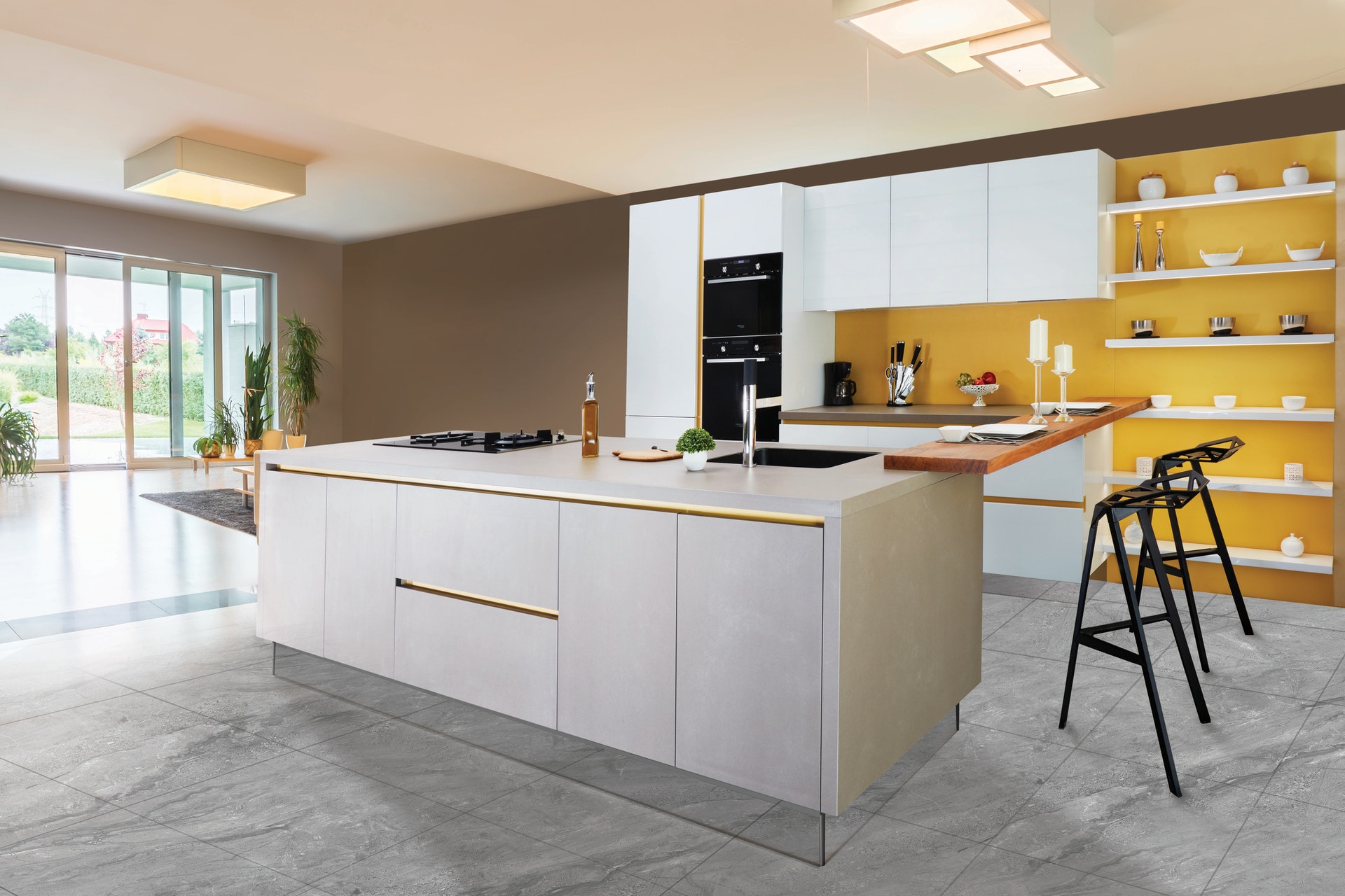
Low chroma: “Elegance”
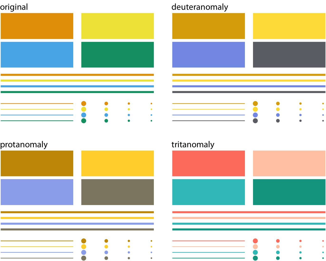
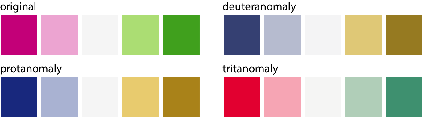
6. Be aware of color-vision deficiency
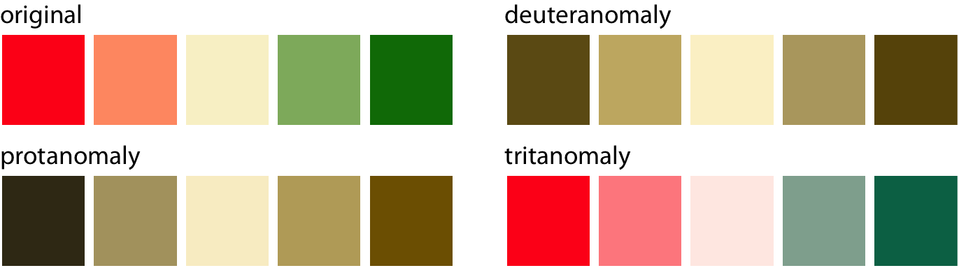
Roughly 5%–8% of men are color blind and 0.5% of women are color blind, with red-green color-vision deficiency being the most common type:
Red-green color-vision deficiency is the most common:
![]()
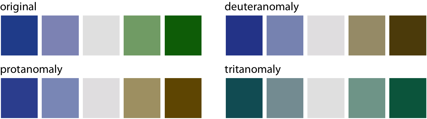
Blue-green color-vision deficiency is rare but does occur:
![]()
Choose colors that can be distinguished with CVD:
![]()
CVD + size
CVD is worse for thin lines and tiny dots
When in doubt, run CVD simulations