Visualizing uncertainty I

Lecture 12

Dr. Mine Çetinkaya-Rundel

Duke University
STA 313 - Spring 2026

Warm up

While you wait

Perceptions of probability

The problem: How do people interpret verbal probability phrases?

“Highly unlikely” vs. “Almost no chance”
“Probable” vs. “Likely”
Do these phrases mean the same thing to everyone?

Two studies:

Heuer (1999): 23 NATO military officers assigned percentages to probability phrases used in intelligence reports
Zonination (2015): Reddit replication with 46 participants – won recognition at 2015 Kantar Information is Beautiful Awards

Heuer (1999)

Davatiz of the day: Zonination (2015)

Announcements

Review quiz feedback – sometimes I leave notes to help you catch up with material you missed
Project 1 presentations on Thursday in lab – be there on time!
Additional OH tomorrow (Tuesday) with me: 10-11:30 Old Chem 211C

Setup

# load packages
library(tidyverse)
library(tidymodels)
library(colorspace)
library(cowplot)
library(distributional)
library(emmeans)
library(ggdist)
library(ggthemes)
library(marginaleffects)
library(ungeviz) # pak::pak("wilkelab/ungeviz")

# set theme for ggplot2
ggplot2::theme_set(ggplot2::theme_minimal(base_size = 16))

# set figure parameters for knitr
knitr::opts_chunk$set(
  fig.width = 7, # 7" width
  fig.asp = 0.618, # the golden ratio
  fig.retina = 3, # dpi multiplier for displaying HTML output on retina
  fig.align = "center", # center align figures
  dpi = 300 # higher dpi, sharper image
)

Probability

Let’s imagine we’re playing a game

The odds are in your favor:
You have a 90% chance of winning!

playing…

Sorry, you lost. 😞

How does that make you feel?

We are bad at judging uncertainty

You had a 10% chance of losing
One in ten playing this game will lose
90% chance of winning is nowhere near a certain win

Visualizing set of possible outcomes

Possible outcomes from 100 individual games played

Frequency framing

This type of visualization is called frequency framing

Uncertainty

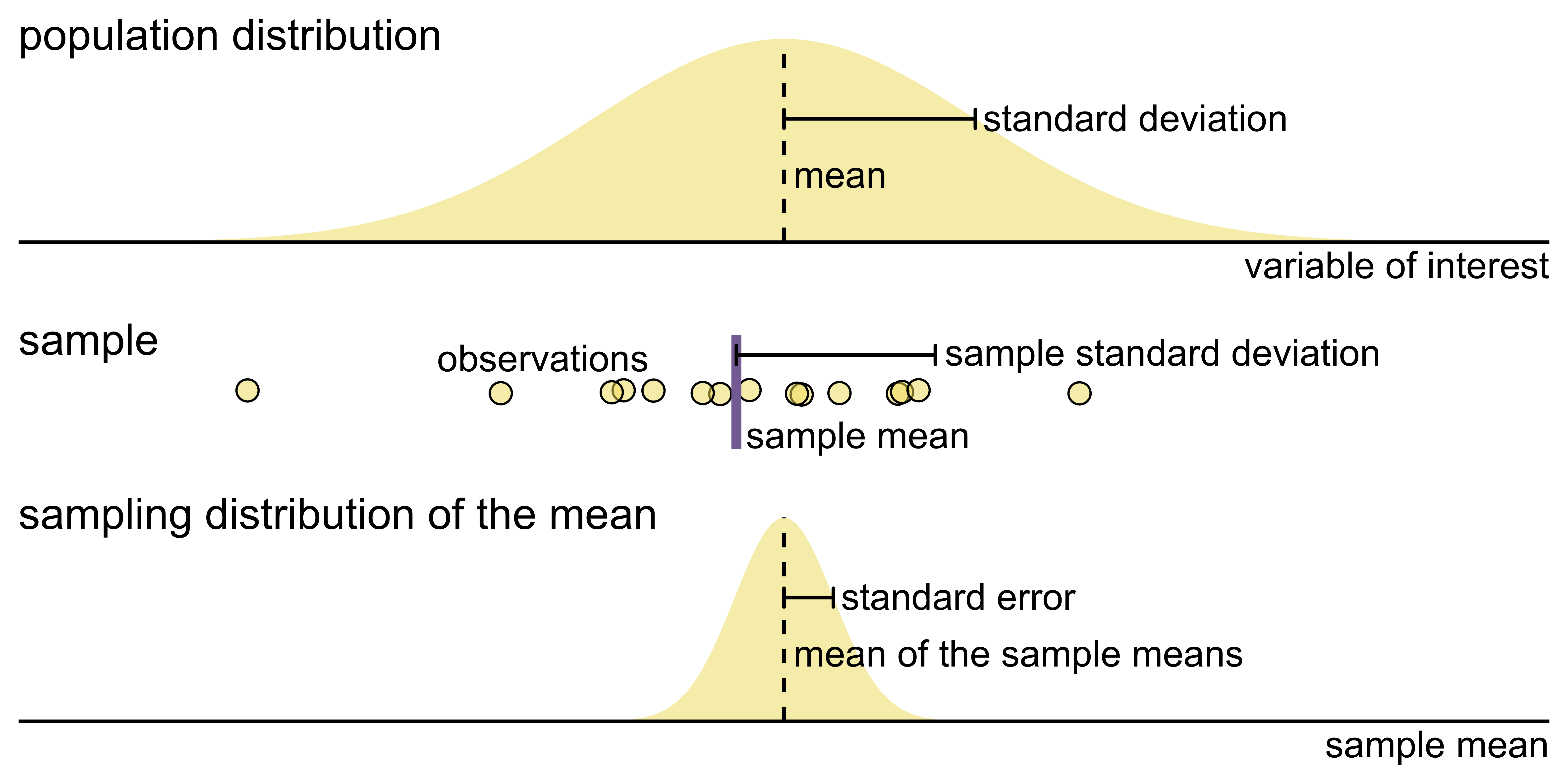
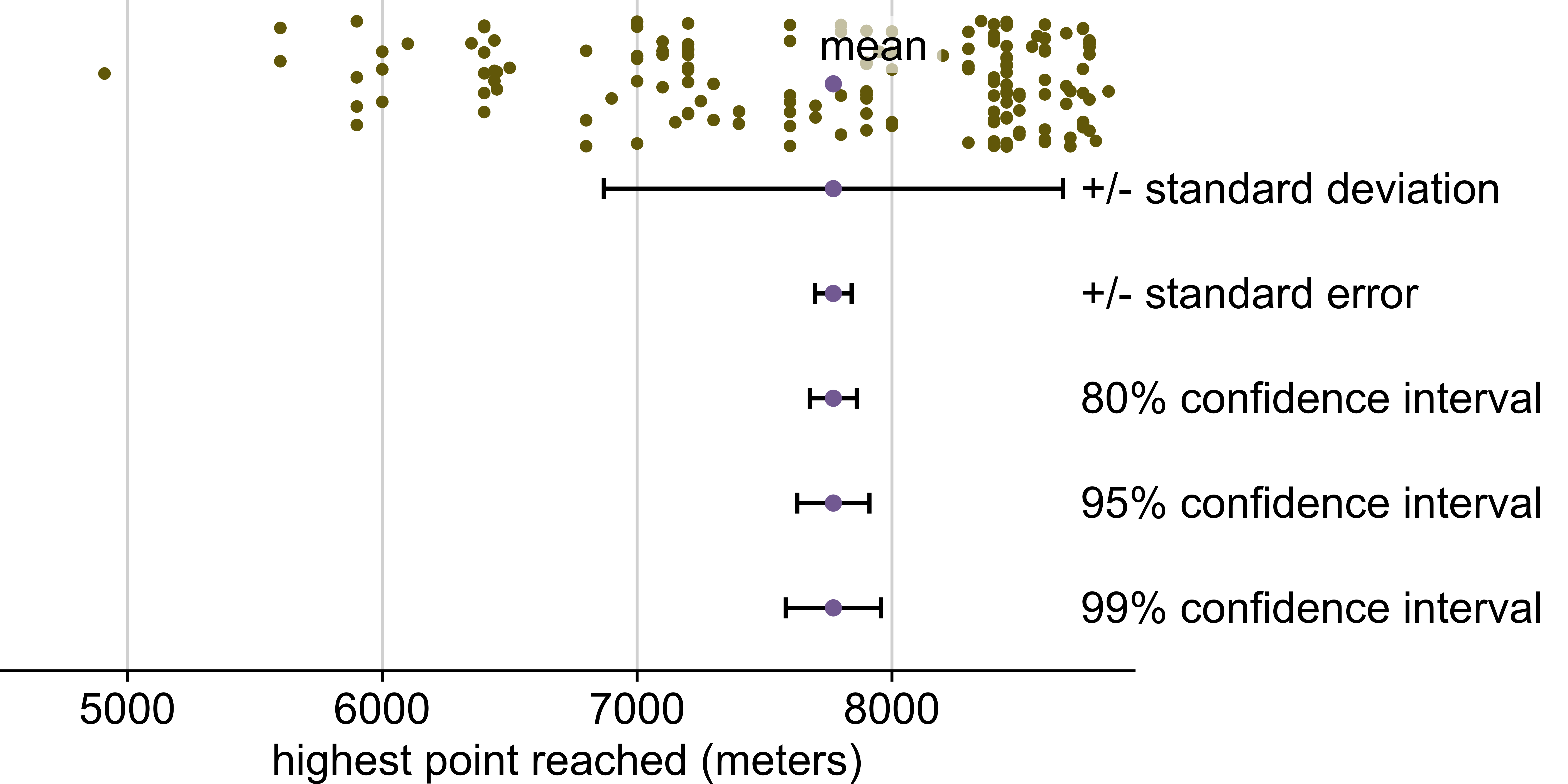
Visualizing uncertainty of point estimates

A point estimate is a single number, such as a mean
Uncertainty is expressed as standard error, confidence interval, or credible interval

Important

Uncertainty of a point estimate != variation in the sample.

Key concepts of statistical sampling

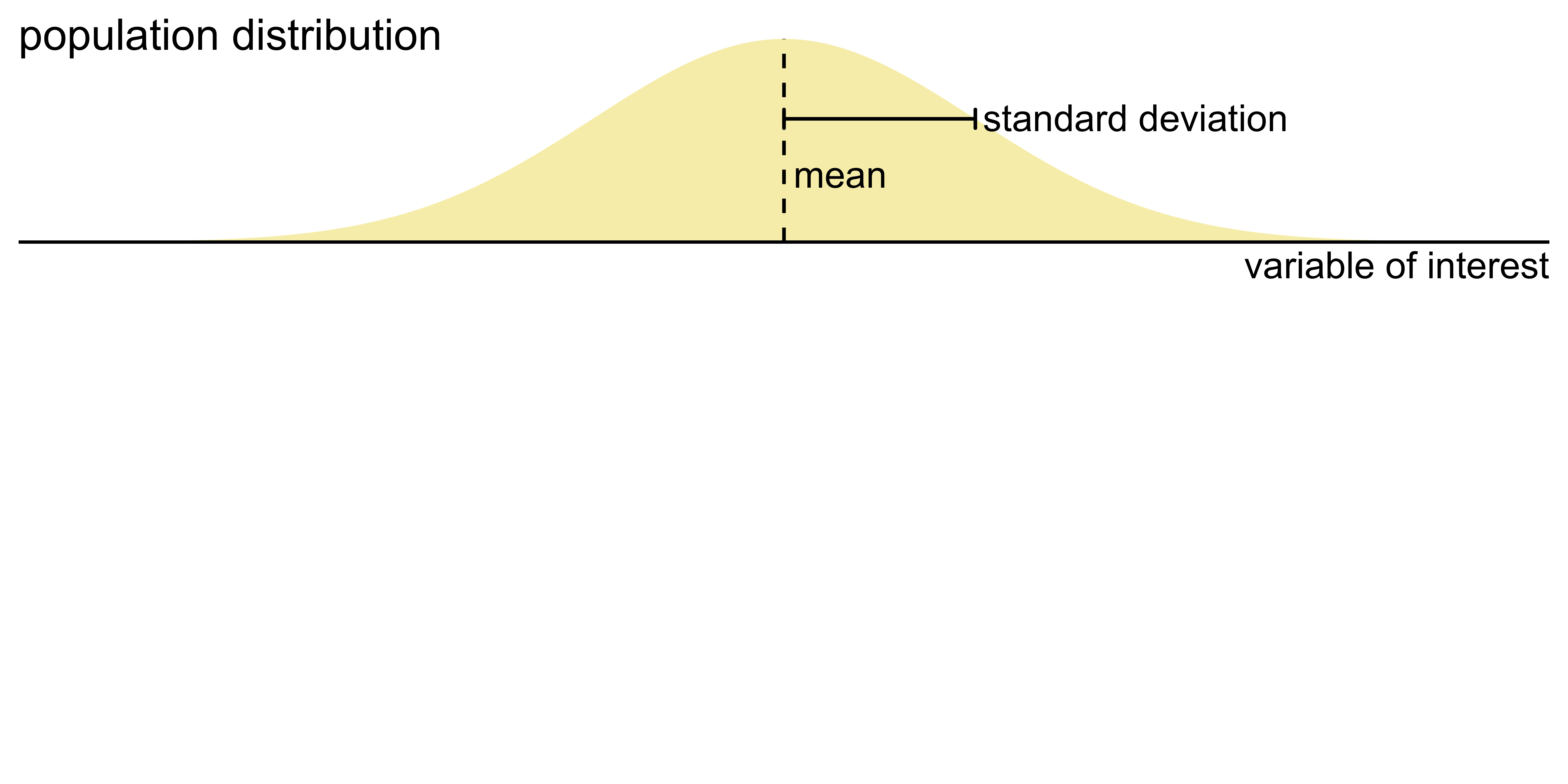
Key concepts of statistical sampling

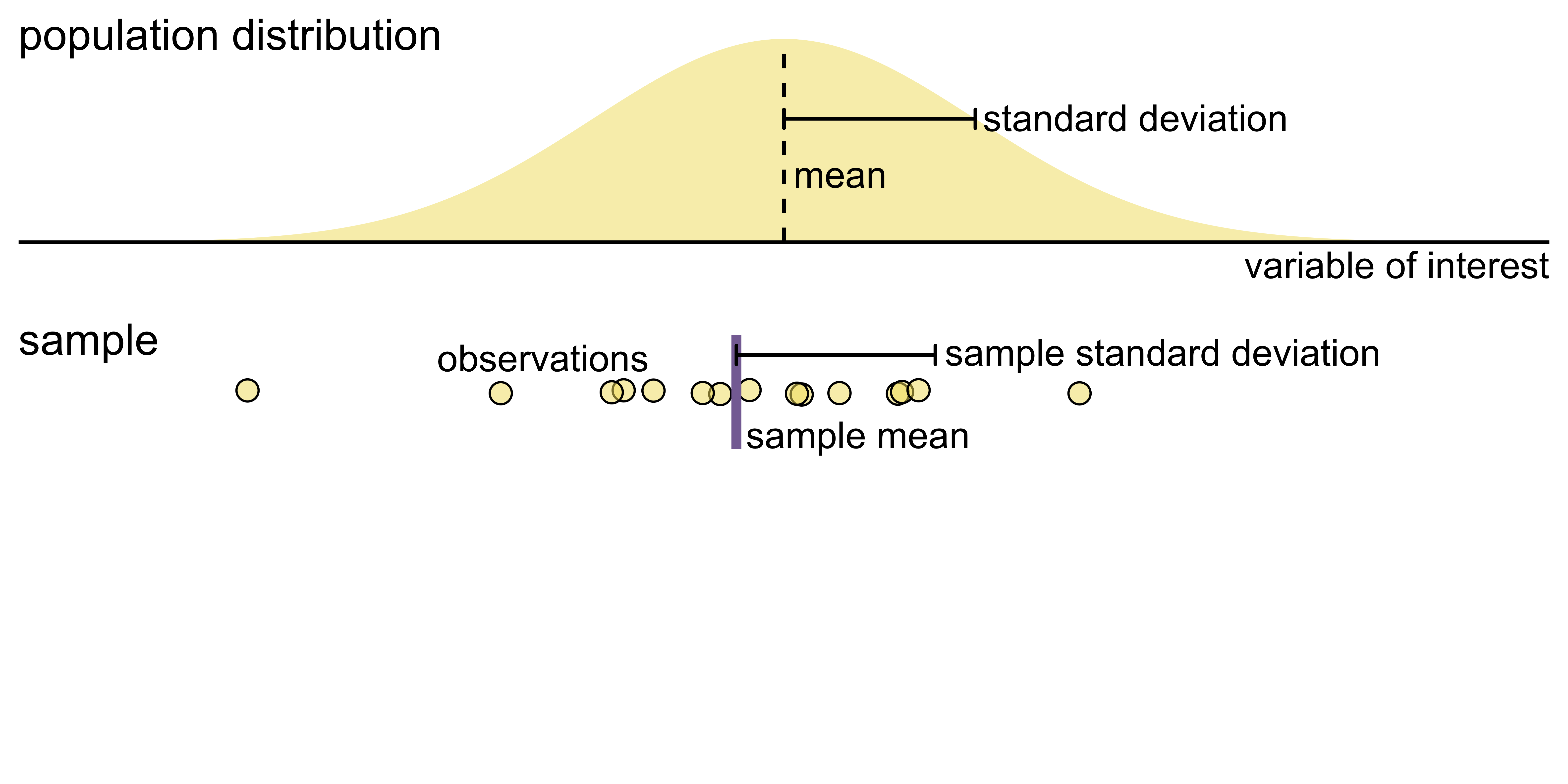
Key concepts of statistical sampling

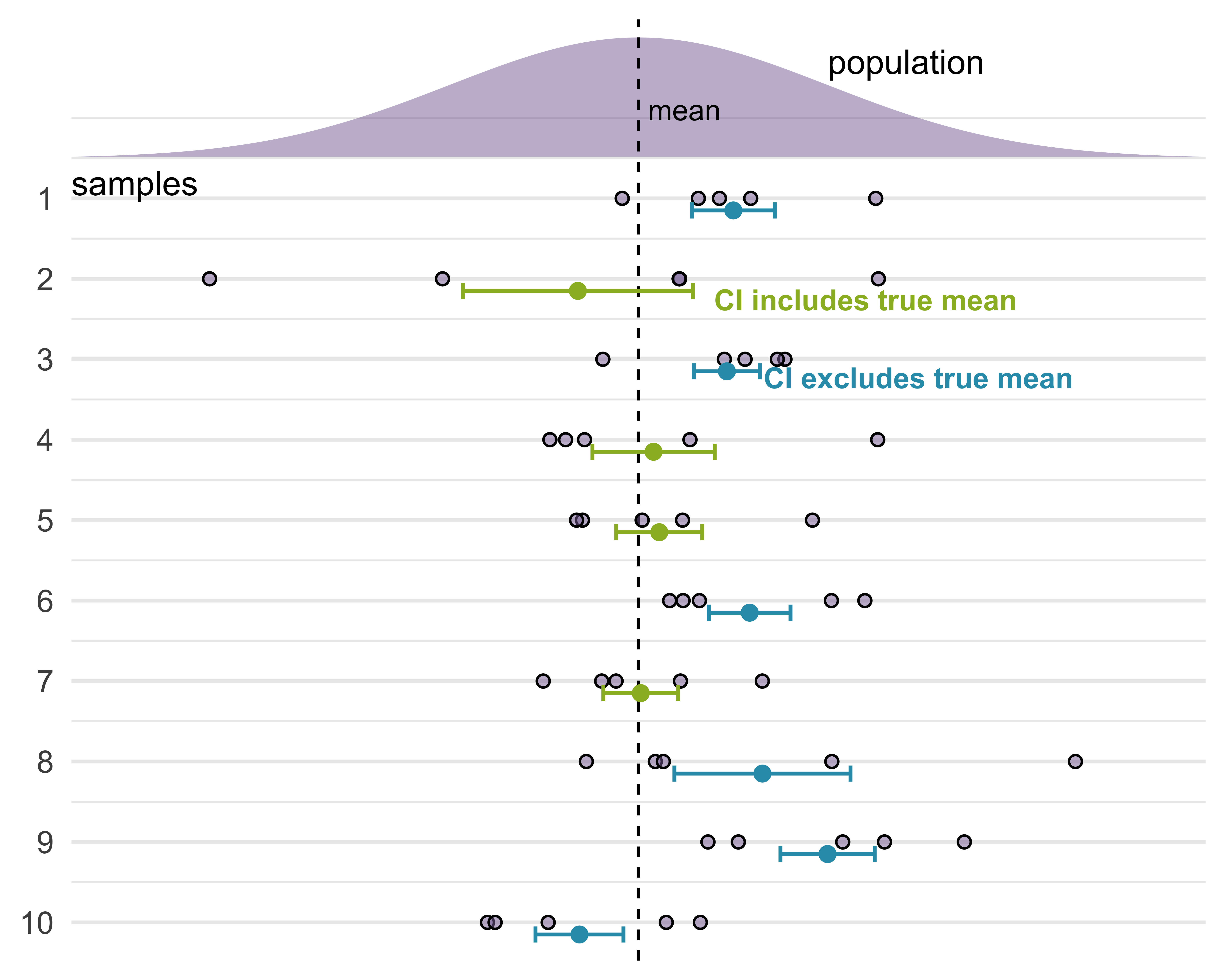
Confidence intervals

What does “95% confident” mean in the following sentence?

We are 95% confident that the confidence interval includes the true population mean.

Confidence intervals

Data: Everest

2019 Everest expedition data from The Himalayan Database via TidyTuesday.

everest_raw <- read_csv("data/everest/everest-2019.csv")

everest_raw

# A tibble: 1,001 × 21
    year expedition_id member_id    highpoint_metres sex   success oxygen_used
   <dbl> <chr>         <chr>                   <dbl> <chr> <chr>   <chr>      
 1  2019 EVER19101     EVER19101-01             8850 Male  Yes     With       
 2  2019 EVER19101     EVER19101-02             8850 Male  Yes     With       
 3  2019 EVER19101     EVER19101-03             8850 Male  Yes     With       
 4  2019 EVER19101     EVER19101-04             8850 Male  Yes     With       
 5  2019 EVER19101     EVER19101-05             8850 Male  Yes     With       
 6  2019 EVER19101     EVER19101-06             8850 Male  Yes     With       
 7  2019 EVER19101     EVER19101-07             8850 Male  Yes     With       
 8  2019 EVER19101     EVER19101-08             8850 Male  Yes     With       
 9  2019 EVER19102     EVER19102-01             8850 Male  Yes     With       
10  2019 EVER19102     EVER19102-02             8850 Male  Yes     With       
# ℹ 991 more rows
# ℹ 14 more variables: peak_id <chr>, peak_name <chr>, season <chr>, age <dbl>,
#   citizenship <chr>, expedition_role <chr>, hired <lgl>, solo <lgl>,
#   died <chr>, death_cause <chr>, death_height_metres <dbl>, injured <lgl>,
#   injury_type <chr>, injury_height_metres <dbl>

Data prep

everest <- everest_raw |>
  mutate(
    died = fct_relevel(died, "No", "Yes"),
    sex = fct_relevel(sex, "Male", "Female"),
    success = fct_relevel(success, "Yes", "No"),
    oxygen_used = fct_relevel(oxygen_used, "With", "Without")
  )

Highest point reached on Everest in 2019

Includes only climbers and expedition members who did not summit

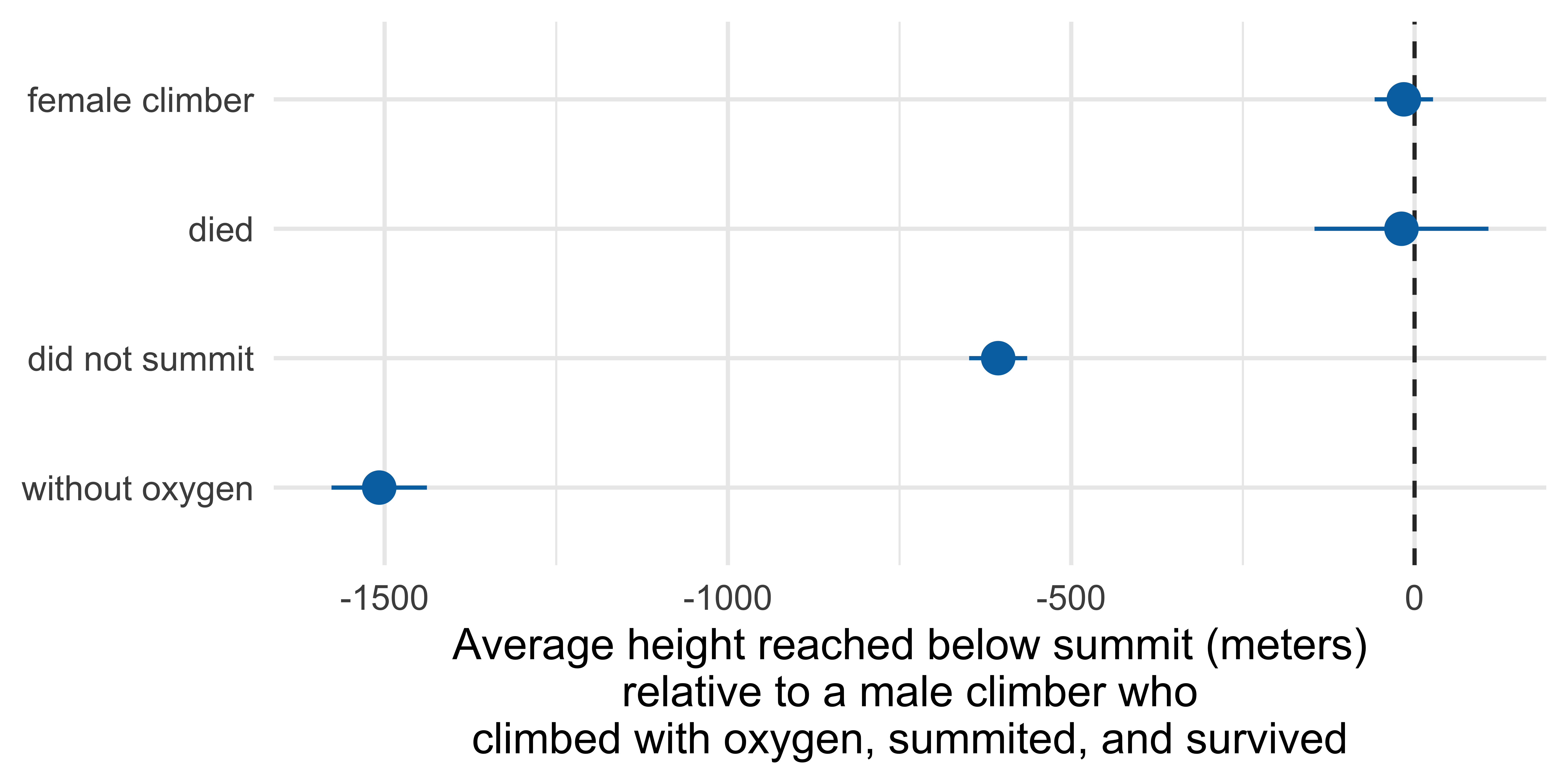
Marginal effects

Marginal effects are the average change in the outcome variable associated with a change in a predictor variable, while holding other variables constant.

Predicting highpoint from…

died, sex, success, and oxygen_used:

everest_fit <- linear_reg() |>
  fit(highpoint_metres ~ died + sex + success + oxygen_used, data = everest)

tidy(everest_fit)

# A tibble: 5 × 5
  term               estimate std.error statistic   p.value
  <chr>                 <dbl>     <dbl>     <dbl>     <dbl>
1 (Intercept)          8855.       7.72  1147.    0        
2 diedYes               -19.1     64.6     -0.295 7.68e-  1
3 sexFemale             -15.6     21.7     -0.720 4.72e-  1
4 successNo            -606.      21.6    -28.1   1.71e-128
5 oxygen_usedWithout  -1508.      35.4    -42.5   3.51e-226

Baseline climber

tidy(everest_fit)

# A tibble: 5 × 5
  term               estimate std.error statistic   p.value
  <chr>                 <dbl>     <dbl>     <dbl>     <dbl>
1 (Intercept)          8855.       7.72  1147.    0        
2 diedYes               -19.1     64.6     -0.295 7.68e-  1
3 sexFemale             -15.6     21.7     -0.720 4.72e-  1
4 successNo            -606.      21.6    -28.1   1.71e-128
5 oxygen_usedWithout  -1508.      35.4    -42.5   3.51e-226

Survived
Male
Climbed with oxygen
Summited

Marginal effects: Height reached on Everest

everest_margins <- avg_comparisons(everest_fit)
everest_margins


        Term       Contrast Estimate Std. Error       z Pr(>|z|)     S   2.5 %
 died        Yes - No          -19.1       64.6  -0.295    0.768   0.4  -145.7
 oxygen_used Without - With  -1507.8       35.4 -42.535   <0.001   Inf -1577.3
 sex         Female - Male     -15.6       21.7  -0.720    0.472   1.1   -58.2
 success     No - Yes         -606.4       21.6 -28.113   <0.001 575.3  -648.7
  97.5 %
   107.6
 -1438.4
    26.9
  -564.1

Type: numeric

Marginal effects to plot

everest_to_plot <- tidy(everest_margins) |>
  mutate(
    factor = fct_reorder(
      fct_recode(
        term,
        "female climber" = "sex",
        "did not summit" = "success",
        "without oxygen" = "oxygen_used"
      ),
      estimate
    )
  )

everest_to_plot

# A tibble: 4 × 10
  term        contrast   estimate std.error statistic   p.value s.value conf.low
  <chr>       <chr>         <dbl>     <dbl>     <dbl>     <dbl>   <dbl>    <dbl>
1 died        Yes - No      -19.1      64.6    -0.295 7.68e-  1   0.381   -146. 
2 oxygen_used Without -…  -1508.       35.4   -42.5   0         Inf      -1577. 
3 sex         Female - …    -15.6      21.7    -0.720 4.72e-  1   1.08     -58.2
4 success     No - Yes     -606.       21.6   -28.1   6.76e-174 575.      -649. 
# ℹ 2 more variables: conf.high <dbl>, factor <fct>

Errorbars

Half-eye

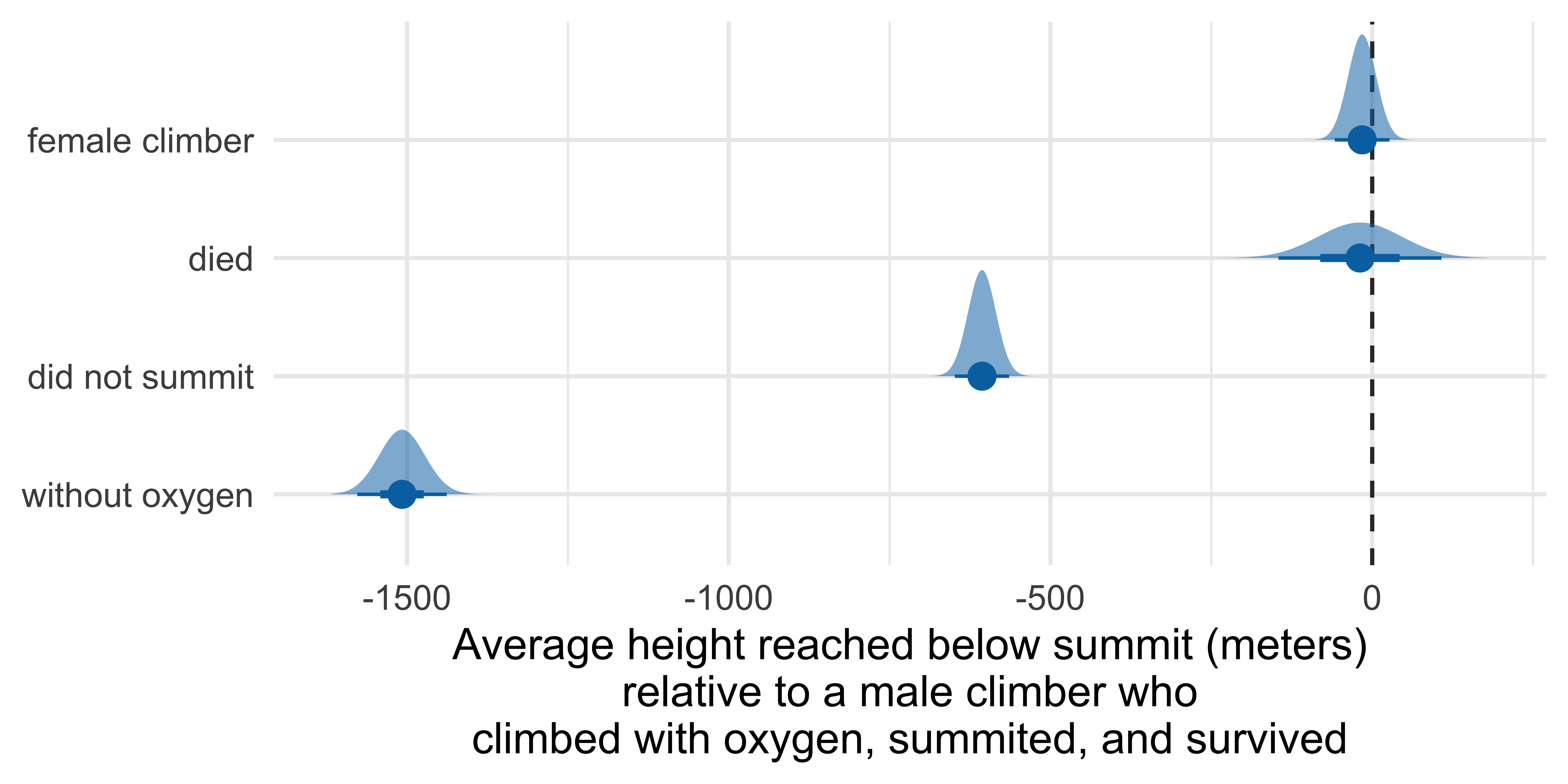
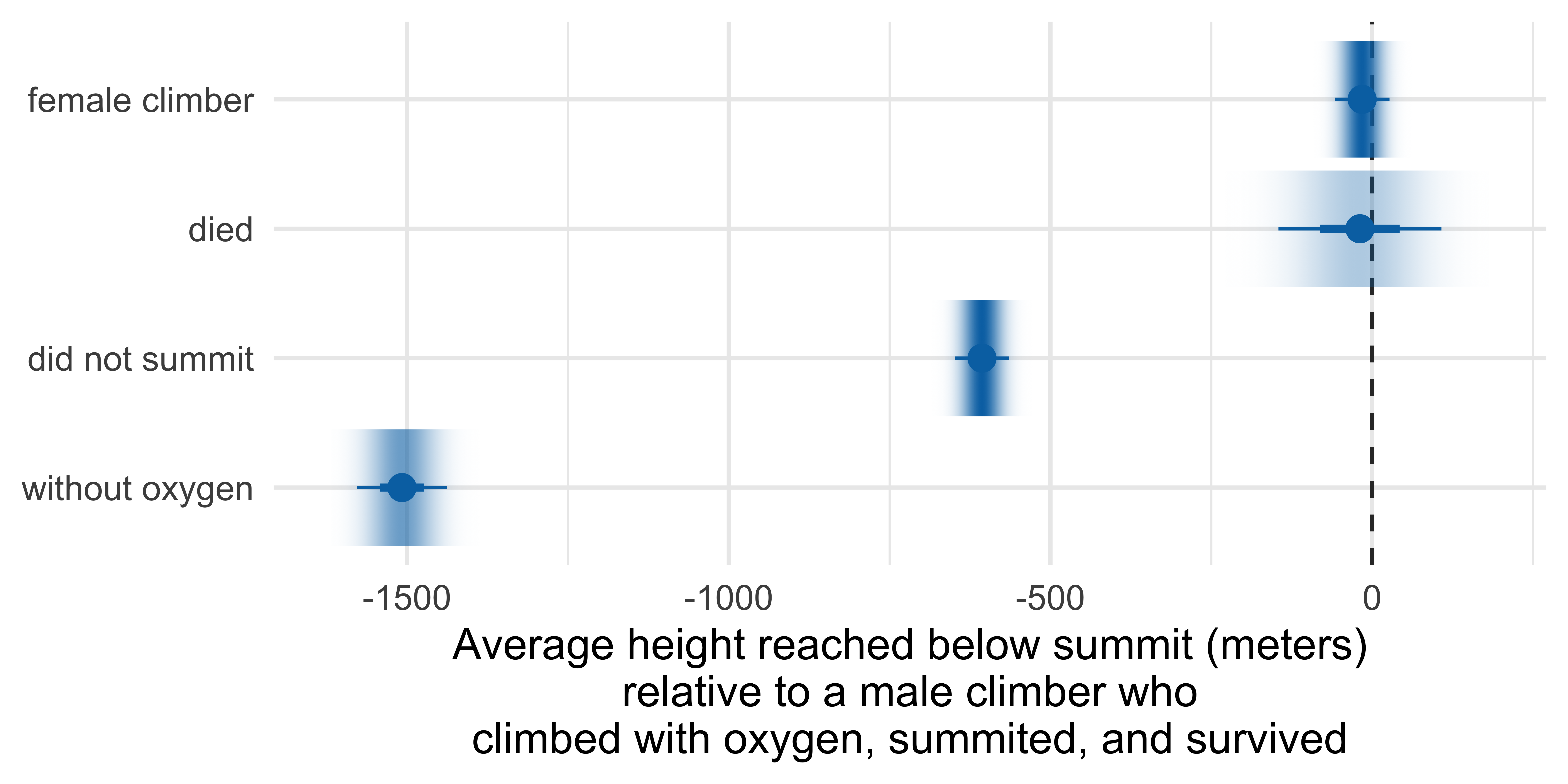
Gradient interval

Quantile dotplot

with fewer quantiles

Quantile dotplot

with more quantiles

Visualizing uncertainty in model estimates

Data: Life expectancy vs. GDP per capita

life_exp_gdp_raw <- read_csv("data/life-exp-gdp/life-exp-gdp.csv")

life_exp_gdp_raw

# A tibble: 3,088 × 5
   country     continent  year life_exp gdp_percap
   <chr>       <chr>     <dbl>    <dbl>      <dbl>
 1 Afghanistan Asia       1950     42.7      1729.
 2 Afghanistan Asia       1955     43.9      2010.
 3 Afghanistan Asia       1960     45.0      2278.
 4 Afghanistan Asia       1965     46.1      2360.
 5 Afghanistan Asia       1970     47.1      2478.
 6 Afghanistan Asia       1975     47.6      2228.
 7 Afghanistan Asia       1980     43.7      2251.
 8 Afghanistan Asia       1985     42.0      3068.
 9 Afghanistan Asia       1990     53.8      2413.
10 Afghanistan Asia       1995     54.3      1689.
# ℹ 3,078 more rows

Data prep

life_exp_gdp <- life_exp_gdp_raw |>
  filter(year %in% seq(1955, 2025, by = 10)) |>
  mutate(
    continent = fct_relevel(
      continent,
      "Africa",
      "Asia",
      "Europe",
      "North America",
      "South America",
      "Oceania"
    )
  )

Life expectancy vs. log GDP per capita

In ae-08, create a visualization that shows the relationship between life expectancy and GDP per capita across continents and years, including error bars to represent uncertainty in the slope lstimates.

Visualizing uncertainty I

Warm up

While you wait

Perceptions of probability

Heuer (1999)

Davatiz of the day: Zonination (2015)

Announcements

Setup

Probability

We are bad at judging uncertainty

Visualizing set of possible outcomes

Frequency framing

Uncertainty

Visualizing uncertainty of point estimates

Key concepts of statistical sampling

Key concepts of statistical sampling

Key concepts of statistical sampling

Confidence intervals

Confidence intervals

Data: Everest

Data prep

Highest point reached on Everest in 2019

Marginal effects

Marginal effects

Predicting highpoint from…

Baseline climber

Marginal effects: Height reached on Everest

Marginal effects to plot

Errorbars

Half-eye

Gradient interval

Quantile dotplot

Quantile dotplot

Quantile dotplot

Visualizing uncertainty in model estimates

Data: Life expectancy vs. GDP per capita

Data prep

Life expectancy vs. log GDP per capita

Life expectancy vs. log GDP per capita

Further reading and acknowledgements