Data wrangling + tidying - I

Lecture 3

Dr. Mine Çetinkaya-Rundel

Duke University
STA 313 - Spring 2024

Warm up

Announcements

  • Project 1 due date move to one 1 week later to accommodate a change in schedule in the library visit / historical data visualizations unit.
  • HW 1 is posted, you will be working on it in lab tomorrow, due on Tue, Jan 30 at 5 pm. To submit, simply push your work to your GitHub repository.

From RQ reflections

  • More on the following upcoming in the class:

    • Scales (e.g., 400000 to 400K), themes and theme features (e.g., moving plot title), faceting
    • Plot sizing for including in a report, slide deck, etc.
  • Which plots to use for numerical vs. categorical variables

  • Strategies for figuring out which function to use

  • Why do we need to set a seed for geom_jitter()?

  • How to choose between fill and color?

  • Review more examples of “bad graphs” with less obvious reasons as to why they are bad – bring your (good and bad) plots to school!

  • Suggestion: Time for random plotting/coding questions during/end of class

Today’s focus

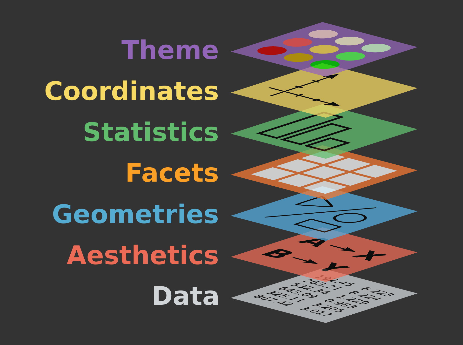
  • Dive into data wrangling and tidying (for better/easier visualization) within a single data frame

  • Peek at one more layer: statistics

    • So far we’ve reviewed data, aesthetics, geometries

    • We’ll soon review facets and themes

    • In your HW you’ll revisit coordinates

Setup

# load packages
library(tidyverse)
library(countdown)
library(scales)
library(ggthemes)
library(glue)
# set theme for ggplot2
ggplot2::theme_set(ggplot2::theme_minimal(base_size = 14))

# set width of code output
options(width = 65)

# set figure parameters for knitr
knitr::opts_chunk$set(
  fig.width = 7, # 7" width
  fig.asp = 0.618, # the golden ratio
  fig.retina = 3, # dpi multiplier for displaying HTML output on retina
  fig.align = "center", # center align figures
  dpi = 300 # higher dpi, sharper image
)

Transforming and reshaping a single data frame

Scenario 1

We…

have a single data frame

want to slice it, and dice it, and juice it, and process it, so we can plot it

Data: Hotel bookings

  • Data from two hotels: one resort and one city hotel
  • Observations: Each row represents a hotel booking
hotels <- read_csv("https://raw.githubusercontent.com/rfordatascience/tidytuesday/master/data/2020/2020-02-11/hotels.csv")
names(hotels)
 [1] "hotel"                          "is_canceled"                   
 [3] "lead_time"                      "arrival_date_year"             
 [5] "arrival_date_month"             "arrival_date_week_number"      
 [7] "arrival_date_day_of_month"      "stays_in_weekend_nights"       
 [9] "stays_in_week_nights"           "adults"                        
[11] "children"                       "babies"                        
[13] "meal"                           "country"                       
[15] "market_segment"                 "distribution_channel"          
[17] "is_repeated_guest"              "previous_cancellations"        
[19] "previous_bookings_not_canceled" "reserved_room_type"            
[21] "assigned_room_type"             "booking_changes"               
[23] "deposit_type"                   "agent"                         
[25] "company"                        "days_in_waiting_list"          
[27] "customer_type"                  "adr"                           
[29] "required_car_parking_spaces"    "total_of_special_requests"     
[31] "reservation_status"             "reservation_status_date"       

dplyr 101

Which of the following (if any) are unfamiliar to you?

  • distinct()
  • select(), relocate()
  • arrange(), arrange(desc())
  • slice(), slice_head(), slice_tail(), slice_sample()
  • filter()
  • mutate()
  • summarize(), count()

Average cost of daily stay

ae-03 - Part 1: Let’s recreate this visualization!
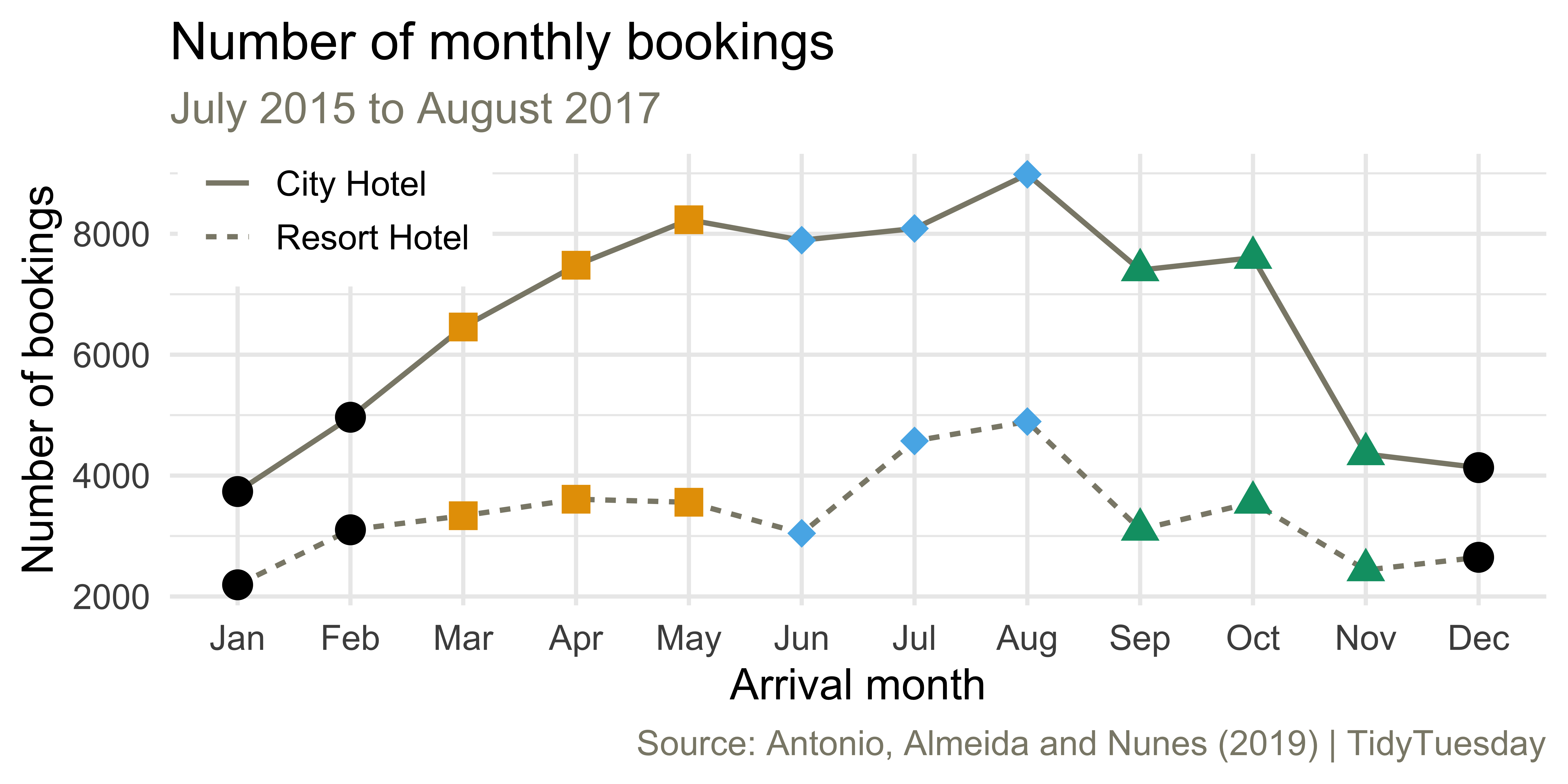
Livecoding

Reveal below for code developed during live coding session.

Code
hotels |>
  mutate(
    arrival_date = glue::glue("{arrival_date_year}-{arrival_date_month}-{arrival_date_day_of_month}"),
    arrival_date = ymd(arrival_date)
  ) |>
  group_by(hotel, arrival_date) |>
  summarise(mean_adr = mean(adr), .groups = "drop") |>
  ggplot(aes(x = arrival_date, y = mean_adr, group = hotel, color = hotel)) +
  geom_line() +
  scale_color_manual(values = c("cornsilk4", "deepskyblue3")) +
  scale_y_continuous(labels = label_dollar()) +
  labs(
    x = "Arrival date",
    y = "Mean average\ndaily rate (USD)",
    color = NULL,
    title = "Cost of daily hotel stay",
    subtitle = "July 2015 to August 2017",
    caption = "Source: Antonio, Almeida and Nunes (2019) | TidyTuesday"
  ) +
  theme(
    legend.position = c(0.15, 0.9),
    legend.box.background = element_rect(
      fill = "white",
      color = "white"
    ),
    plot.subtitle = element_text(color = "cornsilk4"),
    plot.caption = element_text(color = "cornsilk4")
  )

Monthly bookings

Come up with a plan for making the following visualization and write the pseudocode.

Monthly bookings

ae-03 - Part 2: Let’s recreate this visualization!

Livecoding

Reveal below for code developed during live coding session.

Code
hotels <- hotels |>
  mutate(
    arrival_date_month = fct_relevel(arrival_date_month, month.name),
    season = case_when(
      arrival_date_month %in% c("December", "January", "February") ~ "Winter",
      arrival_date_month %in% c("March", "April", "May") ~ "Spring",
      arrival_date_month %in% c("June", "July", "August") ~ "Summer",
      TRUE ~ "Fall"
    ),
    season = fct_relevel(season, "Winter", "Spring", "Summer", "Fall")
  )

hotels |>
  count(season, hotel, arrival_date_month) |>
  ggplot(aes(x = arrival_date_month, y = n, group = hotel, linetype = hotel)) +
  geom_line(linewidth = 0.8, color = "cornsilk4") +
  geom_point(aes(shape = season, color = season), size = 4, show.legend = FALSE) +
  scale_x_discrete(labels = month.abb) +
  scale_color_colorblind() +
  scale_shape_manual(values = c("circle", "square", "diamond", "triangle")) +
  labs(
    x = "Arrival month", y = "Number of bookings", linetype = NULL,
    title = "Number of monthly bookings",
    subtitle = "July 2015 to August 2017",
    caption = "Source: Antonio, Almeida and Nunes (2019) | TidyTuesday"
  ) +
  coord_cartesian(clip = "off") +
  theme(
    legend.position = c(0.12, 0.9),
    legend.box.background = element_rect(fill = "white", color = "white"),
    plot.subtitle = element_text(color = "cornsilk4"),
    plot.caption = element_text(color = "cornsilk4")
  )